State-Space Vector Autoregressions in mvgam

By Nicholas Clark in rstats time-series mvgam

September 6, 2024

Vector Autoregressions (VAR models), also known in the ecological literature as Multivariate Autoregressions (MAR models), are a class of Dynamic Linear Models that offer a principled way to model both delayed and contemporaneous interactions among sets of multiple time series. These models are widely used in econometrics and psychology, among other fields, where they can be analyzed to ask many interesting questions about potential causality, cascading temporal interaction effects or community stability. A VAR(1) model, where temporal interactions among series can take place at a lag of one time step, is defined as:

$$y_t \sim{MVNormal}(\alpha + A * y_{t-1}, \Sigma)$$

Where:

$y_t$ is a vector of time series observations at time $t$
$\alpha$ is a vector of constants capturing the long-term means of each series in $y$
$A$ is a matrix of autoregressive coefficients estimating lagged dependence and cross-dependence between the elements of $y$
$\Sigma$ determines the spread (or flexibility) of the process and any contemporaneous correlations among time series errors

Many R packages exist to estimate parameters of VARs, including the vars and bsvars packages. However, as we can see from the model description above, the traditional VAR model makes two big assumptions: first, this model assumes that the time series being analyzed do not show any measurement error. This assumption may hold for certain types of time series that can be nearly perfectly measured, such as sales of items in a store with accurate digital sale tracking. But it is likely to be broken for the majority of series that are measured with imperfect detectors or with time-varying effort. This can be resolved if we instead refer to a State-Space representation of the model:

Illustration of a basic State-Space model, which assumes that a latent dynamic process (X) can evolve independently from the way we take observations (Y) of that process

A State-Space model is convenient for dealing with many types of real-world time series because they can readily handle observation error, missing values and a broad range of dependency structures. For example, we can modify the VAR(1) described above to a State-Space representation using:

$$y_t \sim{MVNormal}(\alpha + x_t, \Sigma_{obs})$$ $$x_t \sim{MVNormal}(A * x_{t-1}, \Sigma_{process})$$ Where the observation time series $y_t$ are now considered to be noisy observations of some latent $process$ (labelled as $x_t$) and it is this $process$ that evolves as a Vector Autoregression. The advantage of this model is that we can separately estimate process and observation errors (modelled using the two $\Sigma$ matrices). This type of formulation is available using the MARSS package, which has a wonderfully detailed list of worked examples to showcase how flexible and useful these models are.

But the above approach does not address the second major limitation of traditional VARS, which is that they assume that the observation series can be captured with a Gaussian observation model. This makes it difficult to fit VARs to many real-world time series such as counts of multiple species over time, time series of non-negative rates or proportions of customers that responded to a set of surveys. It turns out that this limitation is a much bigger issue when it comes to fitting VARs to real-world data. At the time of writing I could not find a single R package that makes these models accessible, apart from my mvgam package. Given that the question of how to fit time series models to non-Gaussian observations comes up again and again and again (and again), often with unsatisfying answers, this post will demonstrate how the mvgam package can fill this gap. Herein I will show how the package can be used to fit complex multivariate autoregressive models to non-Gaussian time series and how to interrogate the models to ask insightful questions about temporal interactions, variance decompositions and community stability.

Environment setup

This tutorial relies on the following packages (note that mvgam version 1.1.3 or higher is required to carry out these analyses):

library(mvgam)           # Fit, interrogate and forecast DGAMs
library(tidyverse)       # Tidy and flexible data manipulation
library(ggplot2)         # Flexible plotting
library(tidybayes)       # Graceful plotting of Bayesian posterior estimates
library(farver)          # Colour space manipulations

I also define a few plotting utilities to streamline my analysis workflow

theme_set(theme_classic(base_size = 15,
                        base_family = 'serif'))
myhist = function(...){
  geom_histogram(col = 'white',
                 fill = '#B97C7C', ...)
}
hist_theme = function(){
  theme(axis.line.y = element_blank(),
        axis.ticks.y = element_blank(),
        axis.text.y = element_blank())
}

Load, manipulate and plot the data

We will work with a set of annual American kestrel (Falco sparverius) abundance time series, which represent adjusted annual counts of this species taken in three adjacent regions of British Columbia, Canada. These data were collected annually, corrected for changes in observer coverage and detectability, and logged. They can be accessed in the MARSS package

load(url('https://github.com/atsa-es/MARSS/raw/master/data/kestrel.rda'))
head(kestrel)

##      Year British.Columbia Alberta Saskatchewan
## [1,] 1969            0.754   0.460        0.000
## [2,] 1970            0.673   0.899        0.192
## [3,] 1971            0.734   1.133        0.280
## [4,] 1972            0.589   0.528        0.386
## [5,] 1973            1.405   0.789        0.451
## [6,] 1974            0.624   0.528        0.234

Arrange the data into a data.frame that spreads the time series observations into a ’long’ format, which is required for mvgam modelling

regions <- c("BC",
             "Alb",
             "Sask")
model_data <- do.call(rbind,
                      lapply(seq_along(regions),
                             function(x){
  data.frame(year = kestrel[, 1],
             # Reverse the logging so that we deal directly 
             # with the detection-adjusted counts
             adj_count = exp(kestrel[, 1 + x]),
             region = regions[x])})) %>%
  # Add series and time indicators for mvgam modelling
  dplyr::mutate(series = as.factor(region),
                time = year)

Inspect the time series data structure

head(model_data)

##   year adj_count region series time
## 1 1969  2.125485     BC     BC 1969
## 2 1970  1.960109     BC     BC 1970
## 3 1971  2.083398     BC     BC 1971
## 4 1972  1.802185     BC     BC 1972
## 5 1973  4.075527     BC     BC 1973
## 6 1974  1.866379     BC     BC 1974

dplyr::glimpse(model_data)

## Rows: 120
## Columns: 5
## $ year      <dbl> 1969, 1970, 1971, 1972, 1973, 1974, 1975, 1976, 1977, 1978, …
## $ adj_count <dbl> 2.125485, 1.960109, 2.083398, 1.802185, 4.075527, 1.866379, …
## $ region    <chr> "BC", "BC", "BC", "BC", "BC", "BC", "BC", "BC", "BC", "BC", …
## $ series    <fct> BC, BC, BC, BC, BC, BC, BC, BC, BC, BC, BC, BC, BC, BC, BC, …
## $ time      <dbl> 1969, 1970, 1971, 1972, 1973, 1974, 1975, 1976, 1977, 1978, …

levels(model_data$series)

## [1] "Alb"  "BC"   "Sask"

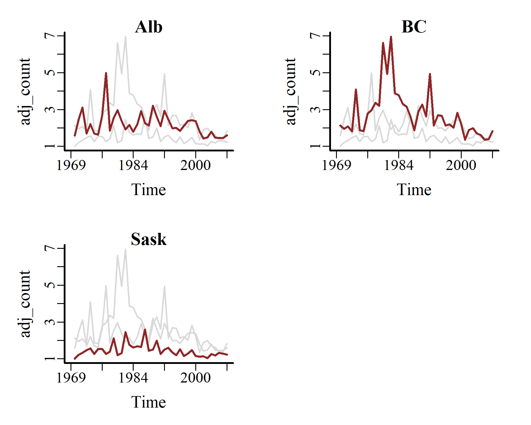
Plot all three the time series together using mvgam’s plot_mvgam_series()

plot_mvgam_series(data = model_data,
                  y = 'adj_count',
                  series = 'all')

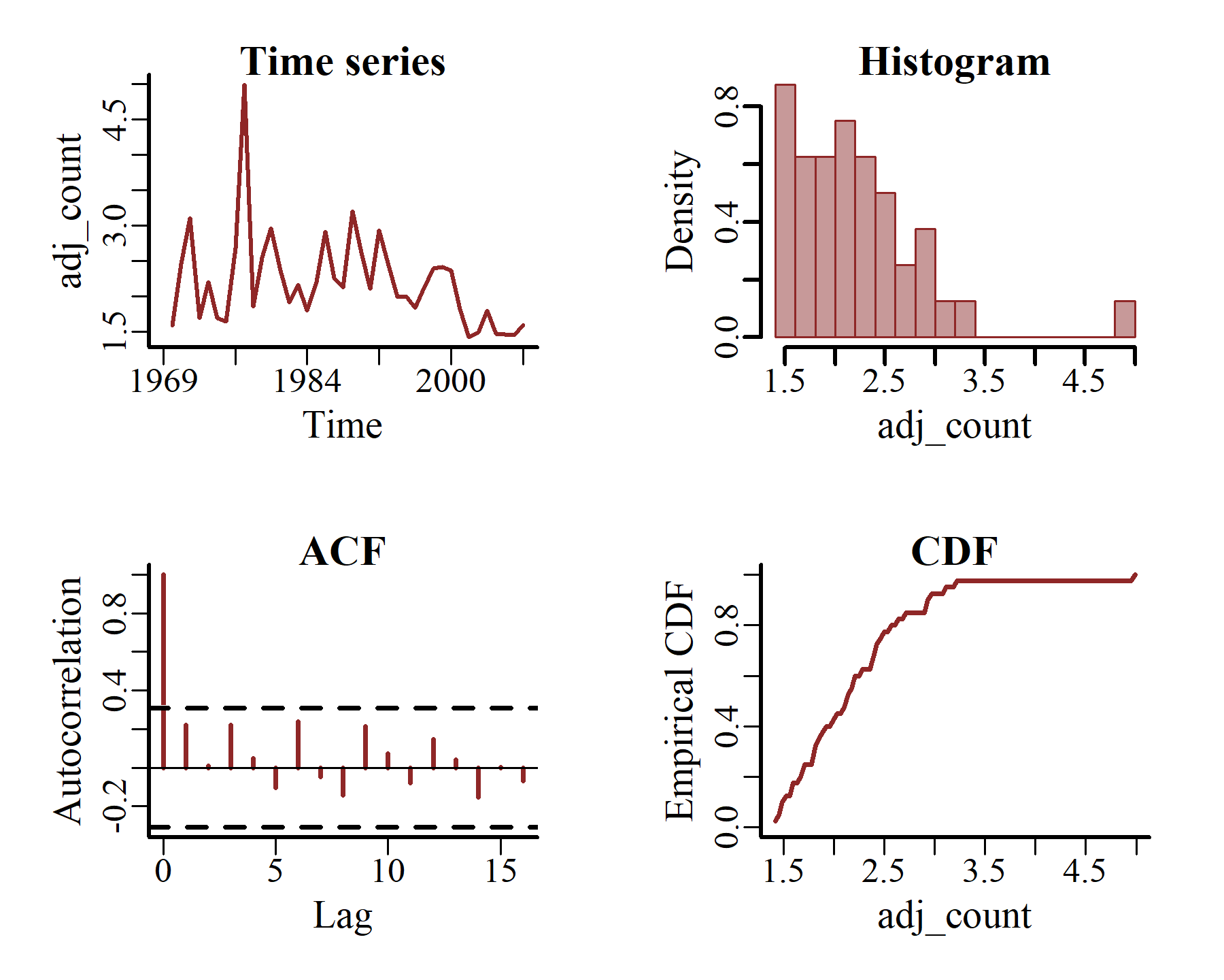
American kestrel adjusted count time series in R

Now plot some additional features, including the empirical CDF and estimated autocorrelation functions, for just one series at a time

plot_mvgam_series(data = model_data,
                  y = 'adj_count',
                  series = 1)

American kestrel time series features in R

plot_mvgam_series(data = model_data,
                  y = 'adj_count',
                  series = 2)

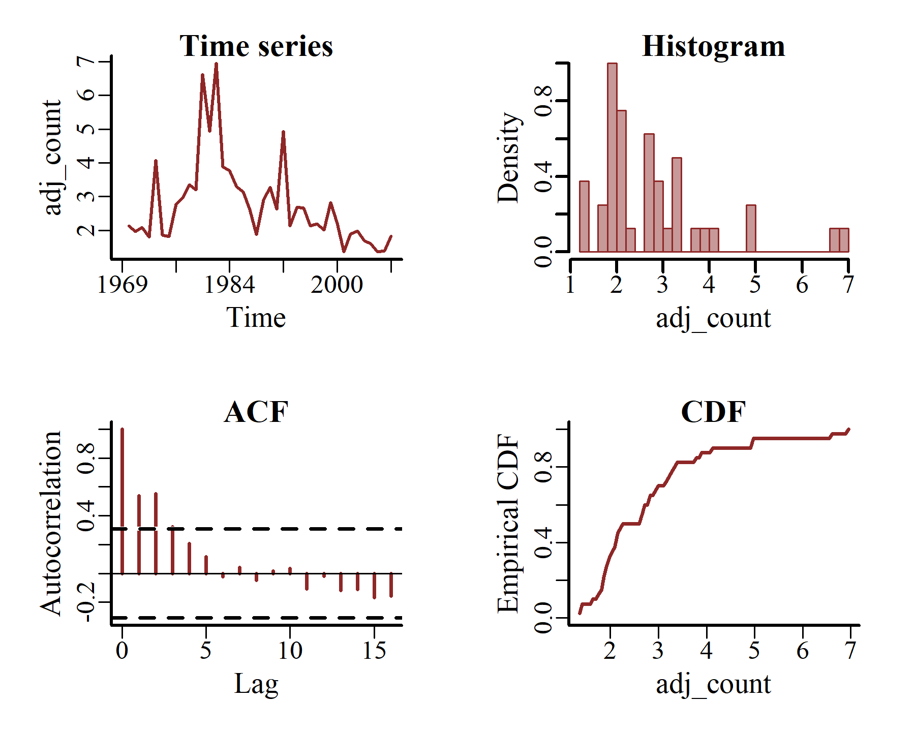
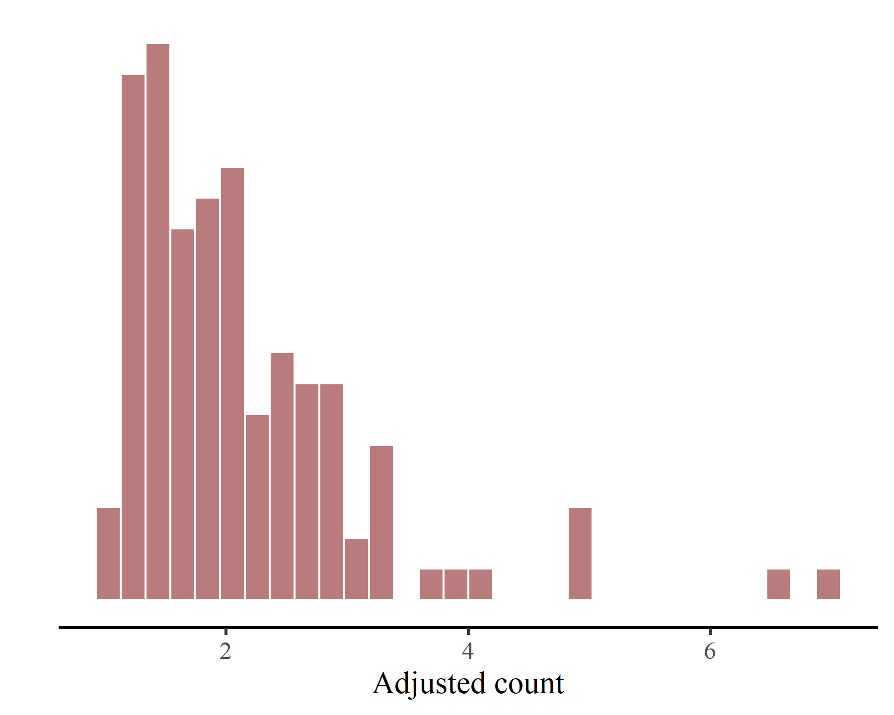
These latter plots make it immediately apparent that our outcome variable, i.e. the adjusted counts of kestrels in each region over time, only takes on non-negative real numbers:

ggplot(model_data,
       aes(x = adj_count)) +
  myhist() +
  labs(x = 'Adjusted count', y = '') +
  hist_theme()

Empirical distribution of American kestrel adjusted counts

Build a State-Space VAR(1) model

Fitting a multivariate time series model to these adjusted counts is not easy using existing R packages. We’d almost certainly have to log-transform the outcome and hope that we don’t lose too much inferential ability in doing so. But, as I’ve shown in other blogposts on this site, there is a better and simpler way to respect the nature of these observations using mvgam. Here we will consider a State-Space model that uses a latent Vector Autoregression as a VAR(1) process. This is done by taking advantage of two key features of the workhorse mvgam() function: First, we can use the trend_formula argument to specify that we want a State-Space model. And second, we can use the trend_model argument to specify that we want the latent process to evolve as a Vector Autoregression of order 1. The mvgam cheatsheet goes into some detail about how each of these arguments work, but your best bet is to read the extensive documentation in ?mvgam::mvgam to fully understand how these models can be constructed. mvgam also takes advantage of a major development in Bayesian VAR modelling, originally published by Sarah Heaps, that enforces stationarity through a principled prior on the autoregressive coefficients. This is extremely helpful for ensuring that we find well-behaving models that don’t give nonsensical and unwieldy forecasts where the forecast variance grows without bound. Given that the average counts of these series seems to vary across regions, we will also want to include region-level intercepts in the process model. And finally, given the nature of the response variable (non-negative real values), a suitable observation family would be the Gamma distribution. First we should inspect default prior distributions for the stochastic parameters involved in our model:

def_priors <- get_mvgam_priors(adj_count ~ -1,
                               trend_formula = ~ region,
                               trend_model = VAR(cor = TRUE),
                               data = model_data,
                               family = Gamma())
def_priors[, 3:4]

##                                           param_info
## 1                                        (Intercept)
## 2                                   process error sd
## 3           diagonal autocorrelation population mean
## 4       off-diagonal autocorrelation population mean
## 5       diagonal autocorrelation population variance
## 6   off-diagonal autocorrelation population variance
## 7      shape1 for diagonal autocorrelation precision
## 8  shape1 for off-diagonal autocorrelation precision
## 9      shape2 for diagonal autocorrelation precision
## 10 shape2 for off-diagonal autocorrelation precision
## 11                             Gamma shape parameter
## 12                         (Intercept) for the trend
## 13                             regionBC fixed effect
## 14                           regionSask fixed effect
##                                      prior
## 1    (Intercept) ~ student_t(3, 0.6, 2.5);
## 2            sigma ~ student_t(3, 0, 2.5);
## 3                               es[1] = 0;
## 4                               es[2] = 0;
## 5                     fs[1] = sqrt(0.455);
## 6                     fs[2] = sqrt(0.455);
## 7                           gs[1] = 1.365;
## 8                           gs[2] = 1.365;
## 9                        hs[1] = 0.071175;
## 10                       hs[2] = 0.071175;
## 11              shape ~ gamma(0.01, 0.01);
## 12 (Intercept)_trend ~ student_t(3, 0, 2);
## 13    regionBC_trend ~ student_t(3, 0, 2);
## 14  regionSask_trend ~ student_t(3, 0, 2);

The priors for regression coefficients ((Intercept)_trend, regionBC_trend and regionsSask_trend) and for the process variances (sigma, which represent the diagonals of the process error matrix $\Sigma_{process}$) are by default set to be quite vague. It is generally good practice to update these using domain knowledge if you want a model that is well-behaved and computationally efficient. Given that the adjusted counts are fairly small and that the Gamma distribution in mvgam uses a log-link function, we don’t expect massive effect sizes in the linear predictor so a more suitable priors for the regression coefficients would be Standard Normal (i.e. $\beta \sim Normal(0, 1)$). We can also change the default half-T prior on the process variances to an Exponential prior that places less belief on extremely large variances. We will leave the priors for the Gamma shape parameter and for the autoregressive partial autocorrelations (which are described in detail by Sarah Heaps in her wonderful VAR stationarity paper) as default. So our first model to consider is:

varmod <- mvgam(
  # Observation formula, empty to only consider the Gamma observation process
  formula = adj_count ~ -1,
  
  # Process model formula that includes regional intercepts 
  trend_formula = ~ region,
  
  # A VAR(1) dynamic process with fully parameterized covariance matrix Sigma
  trend_model = VAR(cor = TRUE),
  
  # Modified prior distributions using brms::prior()
  priors = c(prior(std_normal(), class = Intercept_trend),
             prior(std_normal(), class = b),
             prior(exponential(2.5), class = sigma)),
  
  # The time series data in 'long' format
  data = model_data,
  
  # A Gamma observation family
  family = Gamma(),
  
  # Forcing all three series to share the same Gamma shape parameter
  share_obs_params = TRUE,
  
  # Stan control arguments
  adapt_delta = 0.95,
  burnin = 1000,
  samples = 1000,
  silent = 2)

Model diagnostics and inferences

This model only takes a few seconds to fit four parallel Hamiltonian Monte Carlo chains, though we do get some minor warnings about a few Hamiltonian Monte Carlo divergences which I have mostly mitigated by setting adapt_delta = 0.95:

summary(varmod)

## GAM observation formula:
## adj_count ~ 1
## 
## GAM process formula:
## ~region
## 
## Family:
## Gamma
## 
## Link function:
## log
## 
## Trend model:
## VAR(cor = TRUE)
## 
## N process models:
## 3 
## 
## N series:
## 3 
## 
## N timepoints:
## 40 
## 
## Status:
## Fitted using Stan 
## 4 chains, each with iter = 2000; warmup = 1000; thin = 1 
## Total post-warmup draws = 4000
## 
## 
## Observation shape parameter estimates:
##       2.5% 50% 97.5% Rhat n_eff
## shape   20  33    59 1.02   237
## 
## GAM observation model coefficient (beta) estimates:
##             2.5% 50% 97.5% Rhat n_eff
## (Intercept)    0   0     0  NaN   NaN
## 
## Process model VAR parameter estimates:
##         2.5%    50% 97.5% Rhat n_eff
## A[1,1] -0.02  0.580  1.10 1.01   351
## A[1,2] -0.55 -0.039  0.25 1.01   534
## A[1,3] -0.10  0.540  2.20 1.02   461
## A[2,1] -0.26  0.320  2.00 1.05    84
## A[2,2] -0.78  0.400  0.85 1.02   153
## A[2,3] -0.31  0.690  3.50 1.02   227
## A[3,1] -0.11  0.120  0.78 1.02   182
## A[3,2] -0.22  0.030  0.22 1.01   255
## A[3,3]  0.15  0.640  1.10 1.01   529
## 
## Process error parameter estimates:
##               2.5%      50%  97.5% Rhat n_eff
## Sigma[1,1]  0.0040  0.02100 0.0580 1.01   372
## Sigma[1,2] -0.0068  0.00920 0.0330 1.00   953
## Sigma[1,3] -0.0110 -0.00042 0.0079 1.00   772
## Sigma[2,1] -0.0068  0.00920 0.0330 1.00   953
## Sigma[2,2]  0.0200  0.05000 0.1000 1.01   732
## Sigma[2,3] -0.0065  0.00460 0.0190 1.00  1097
## Sigma[3,1] -0.0110 -0.00042 0.0079 1.00   772
## Sigma[3,2] -0.0065  0.00460 0.0190 1.00  1097
## Sigma[3,3]  0.0012  0.00570 0.0230 1.03   260
## 
## GAM process model coefficient (beta) estimates:
##                    2.5%   50% 97.5% Rhat n_eff
## (Intercept)_trend  0.35  0.70  0.97    1  1296
## regionBC_trend    -0.13  0.14  0.35    1   825
## regionSask_trend  -0.56 -0.39 -0.20    1   941
## 
## Stan MCMC diagnostics:
## n_eff / iter looks reasonable for all parameters
## Rhats above 1.05 found for 1 parameters
##  *Diagnose further to investigate why the chains have not mixed
## 95 of 4000 iterations ended with a divergence (2.375%)
##  *Try running with larger adapt_delta to remove the divergences
## 0 of 4000 iterations saturated the maximum tree depth of 12 (0%)
## E-FMI indicated no pathological behavior
## 
## Samples were drawn using NUTS(diag_e) at Fri Sep 27 12:55:11 PM 2024.
## For each parameter, n_eff is a crude measure of effective sample size,
## and Rhat is the potential scale reduction factor on split MCMC chains
## (at convergence, Rhat = 1)

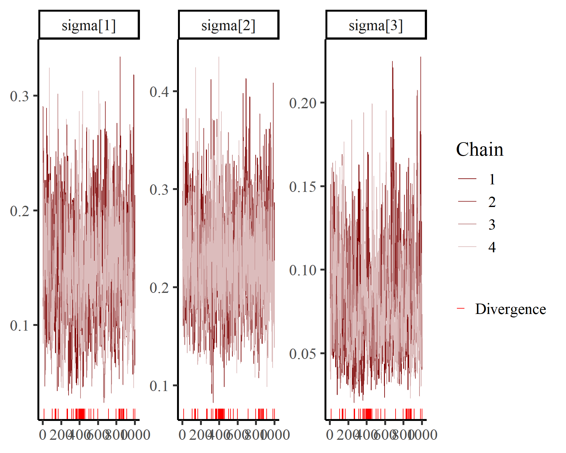
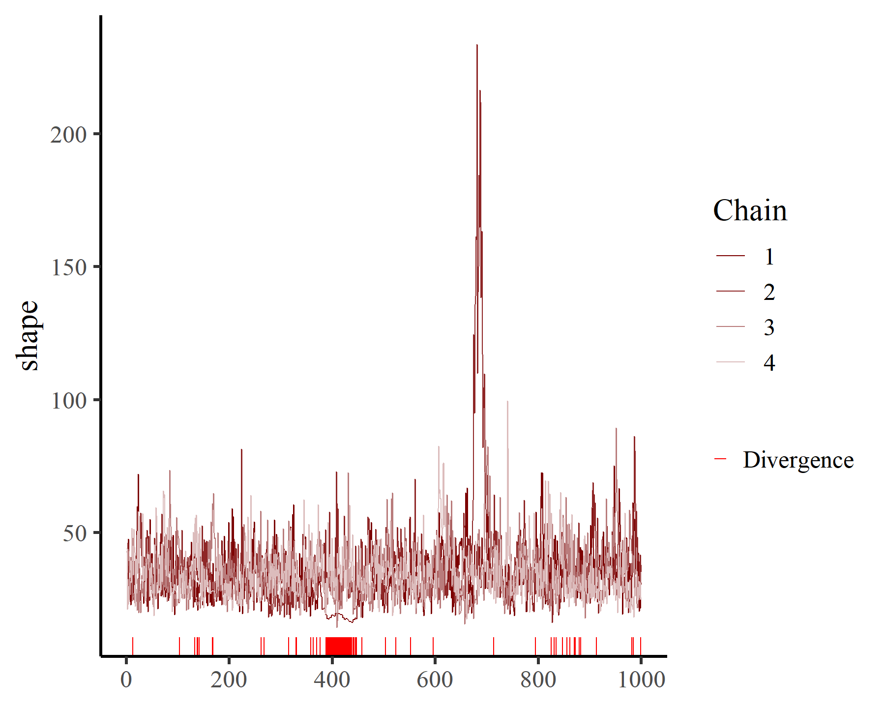
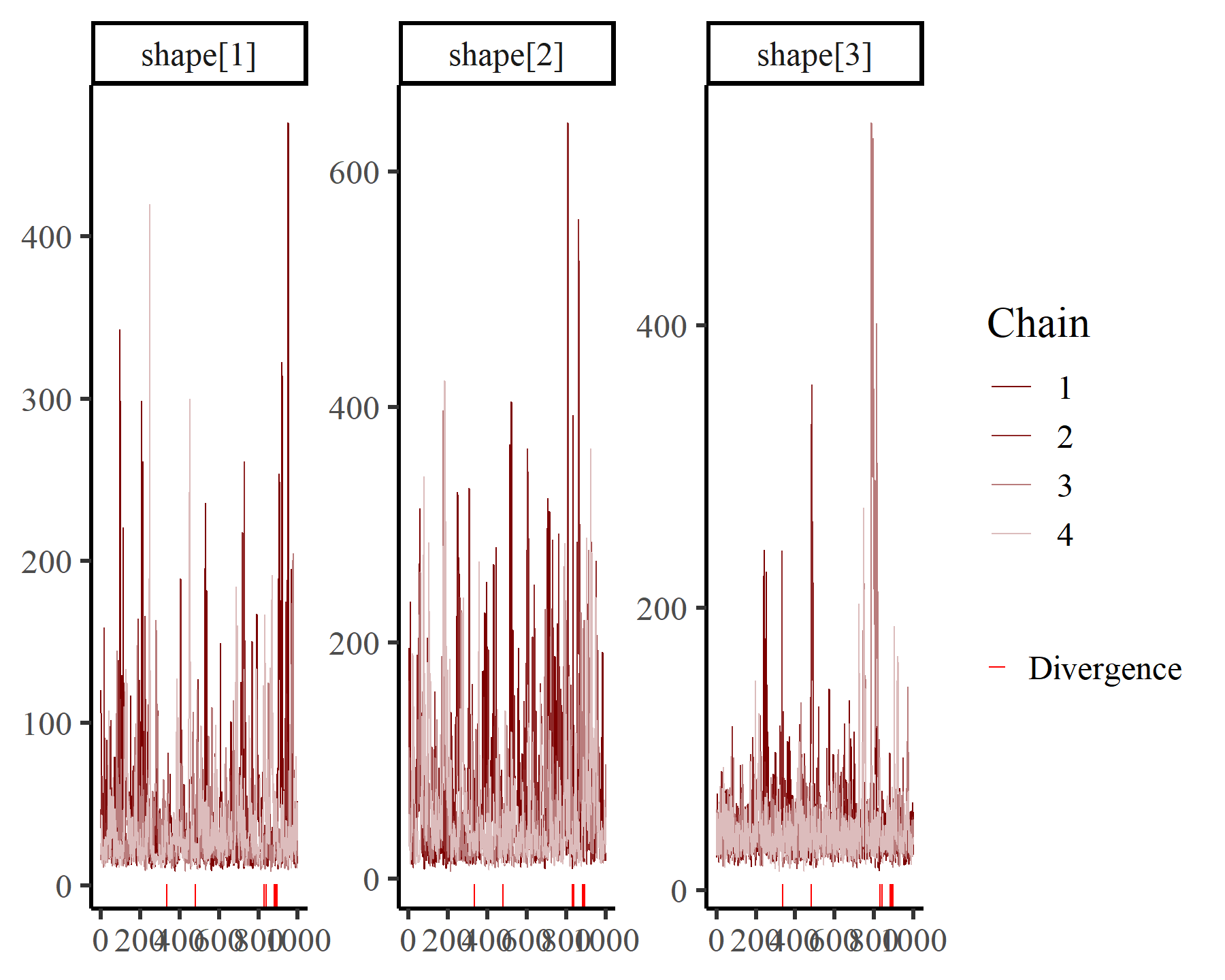
We can inspect posterior estimates for some of the key parameters using bayesplot functionality. For State-Space models, it is particularly recommended to inspect estimates for process and observation scale parameters (labelled as sigma and shape in the model’s MCMC output):

mcmc_plot(varmod,
          variable = 'sigma',
          regex = TRUE,
          type = 'trace')

mvgam posterior estimates using bayesplot

mcmc_plot(varmod,
          variable = 'shape',
          type = 'trace')

Looking at possible coupling between these estimates is also a good idea, which you can do with the pairs() function:

pairs(varmod,
      variable = c('shape', 'sigma'),
      regex = TRUE,
      off_diag_args = list(size = 1,
                           alpha = 0.5))

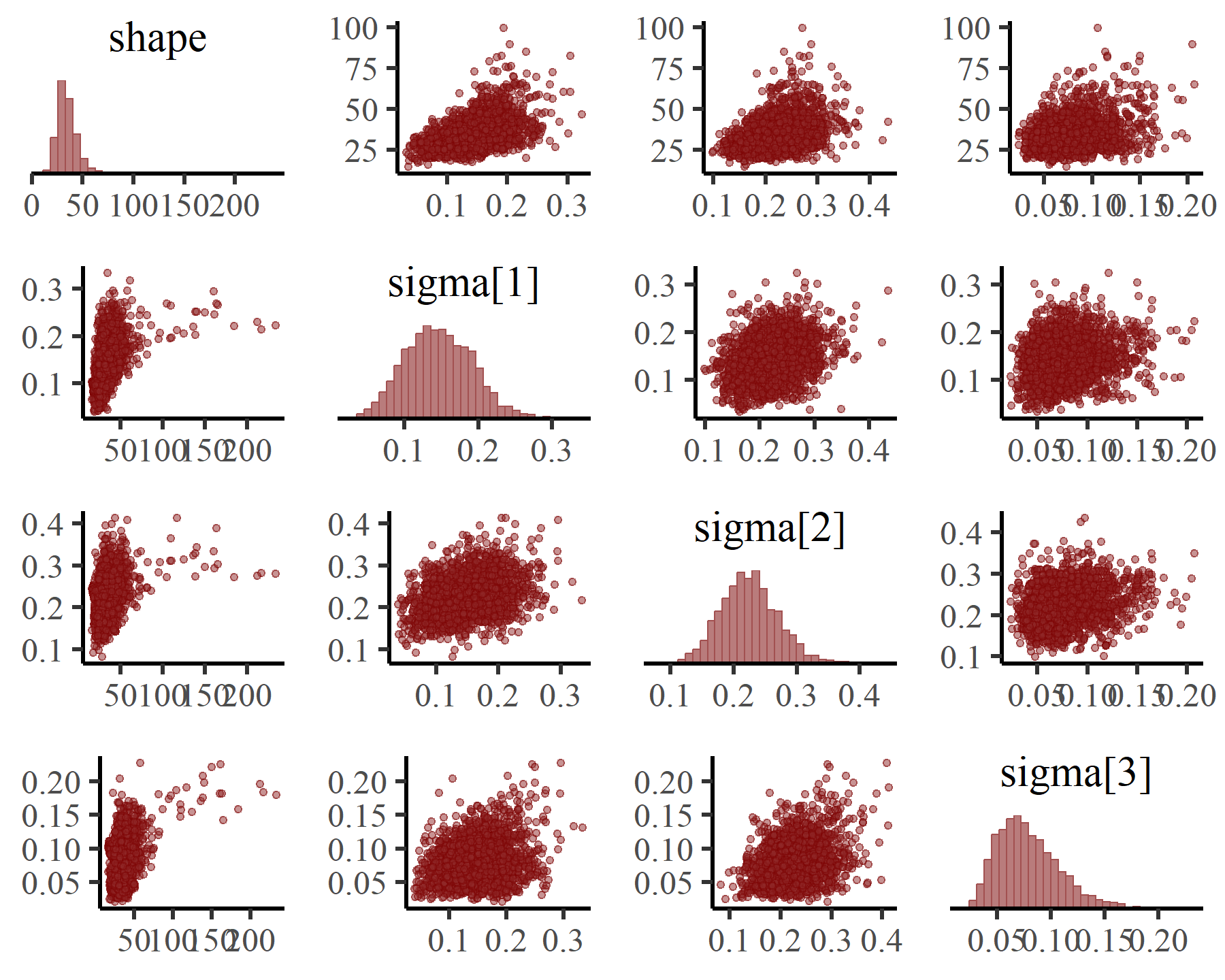
Overall these estimates are quite stable and well-behaved. We can also inspect estimates for any linear predictor effects (in both the process and observation models) using conditional_effects(), which makes use of the wonderful marginaleffects package (see this post on interpreting Generalized Additive Models using marginaleffects for a glimpse into the full power of this package). Since we only have the varying intercepts as regressors in our model, we only get one plot from this call:

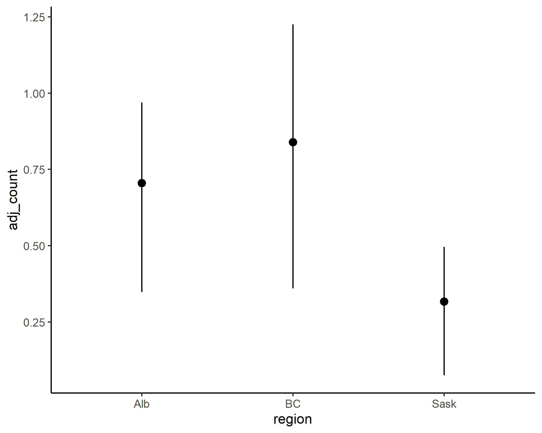
conditional_effects(varmod)

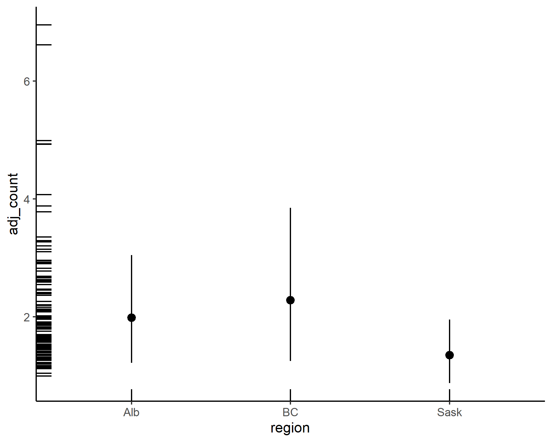
By default conditional_effects() will return predictions on the response scale (i.e. considering the full uncertainty in posterior predictions). But we can also plot these on the link or expectation scales if we wish:

conditional_effects(varmod,
                    type = 'link')

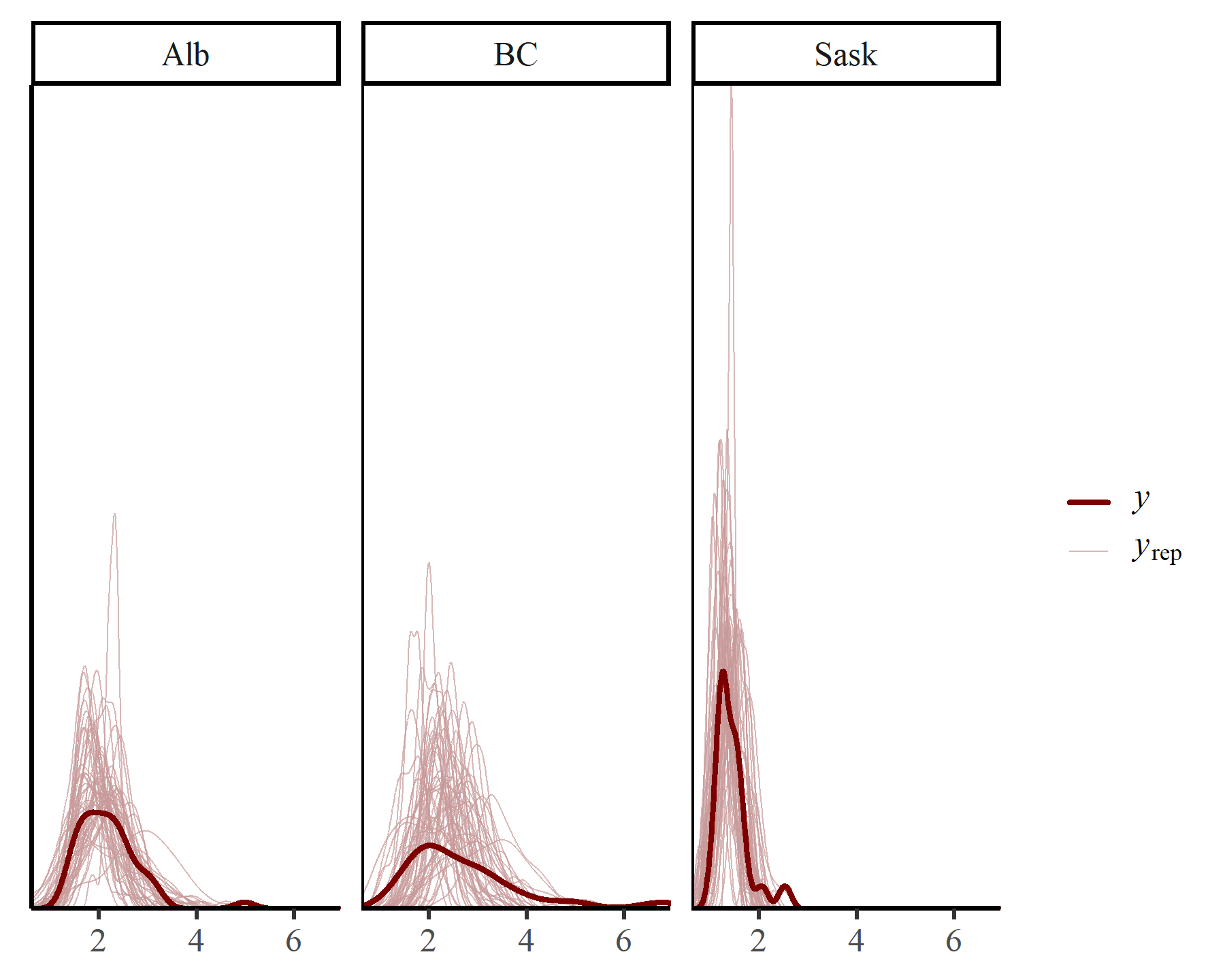
Posterior predictive checks are also useful for interrogating a Bayesian model. mvgam offers multiple ways to do this. First we can compute unconditional posterior predictive checks, which integrate over the possible (stable) temporal states that could have been encountered for each series. In other words, these plots show us the types of predictions that we might make if we had no observations to inform the states of the latent VAR(1) process:

pp_check(varmod,
         type = "dens_overlay_grouped",
         group = "region",
         ndraws = 50)

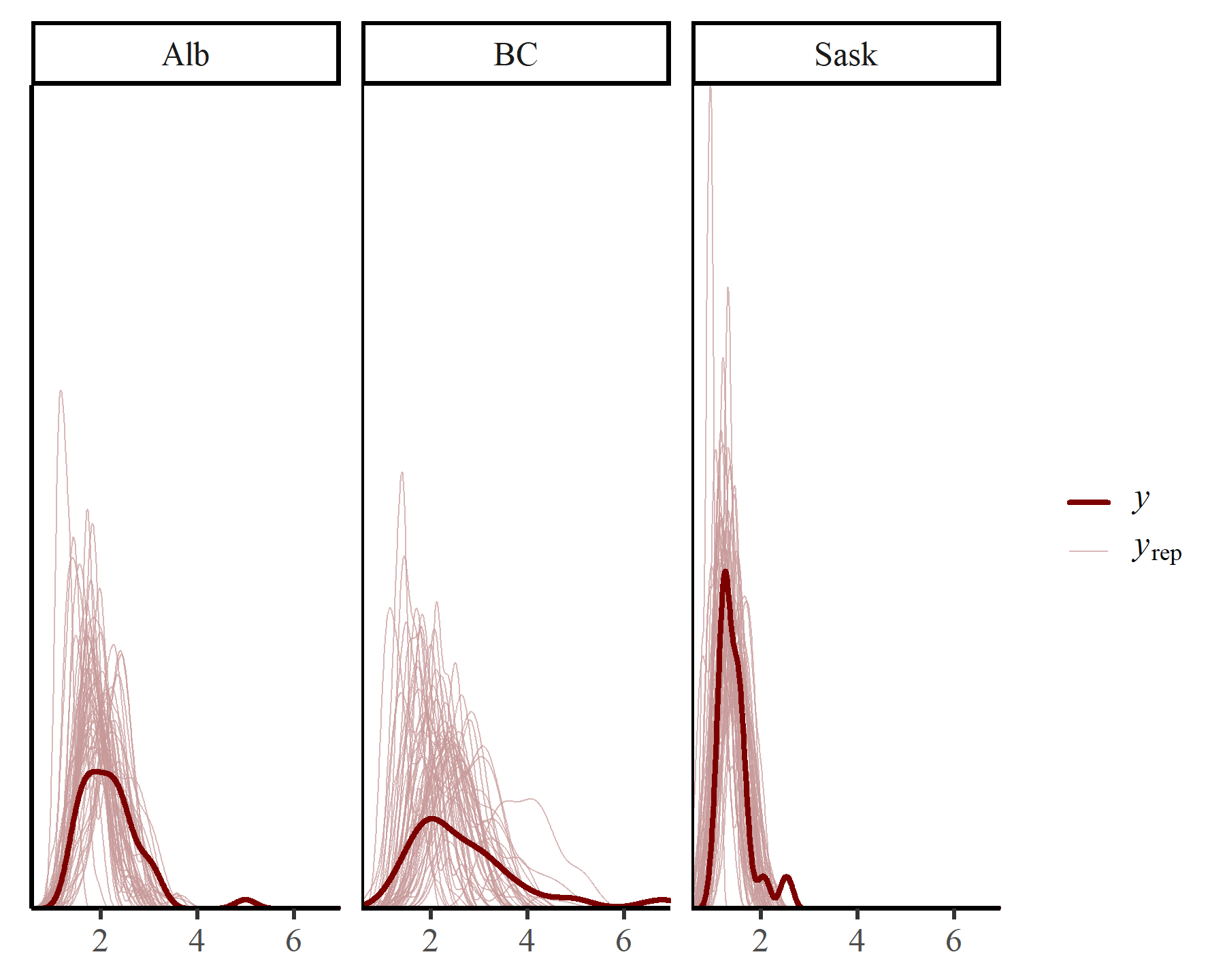
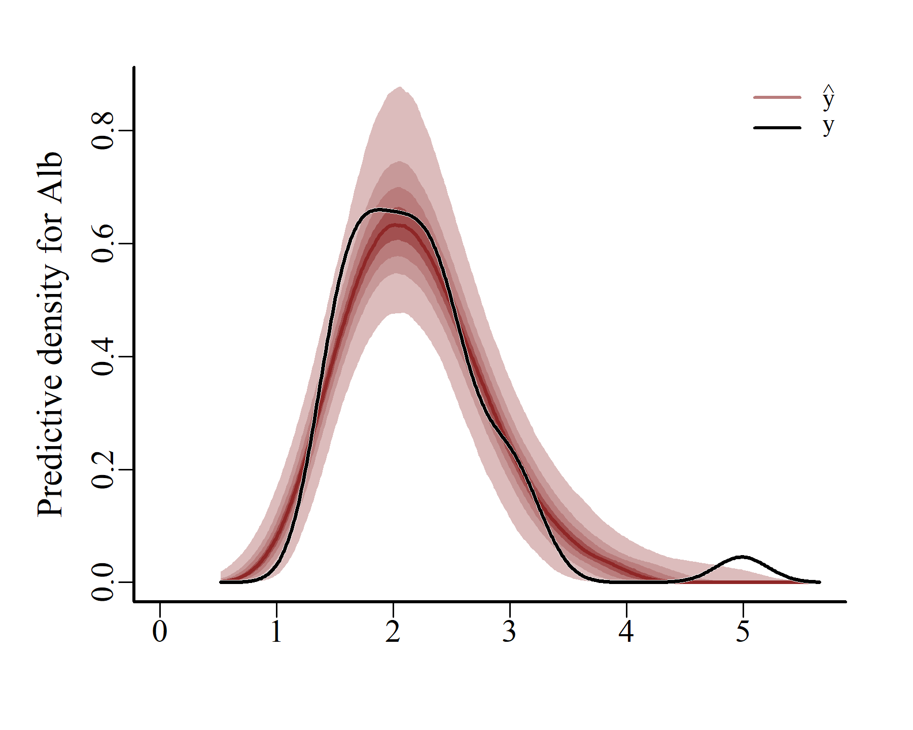
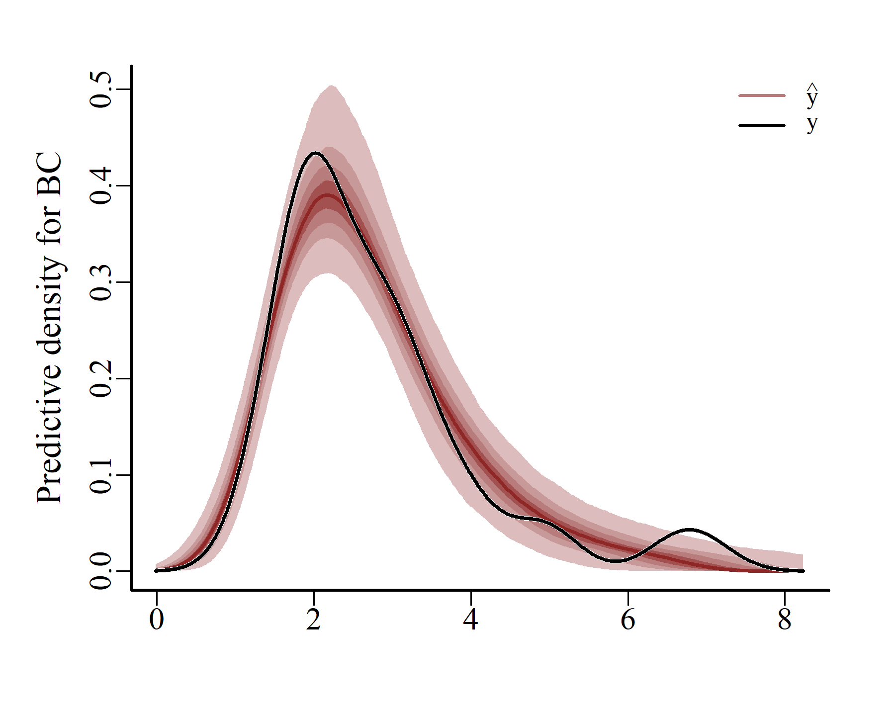
Obviously these prediction densities are more variable than the actual observation densities. But the main shapes seem to have been reasonably well captured. mvgam can also create conditional posterior predictive checks, using the actual latent temporal states that were estimated when the model conditioned on the observed data:

ppc(varmod,
    series = 1,
    type = 'density')

ppc(varmod,
    series = 2,
    type = 'density')

ppc(varmod,
    series = 3,
    type = 'density')

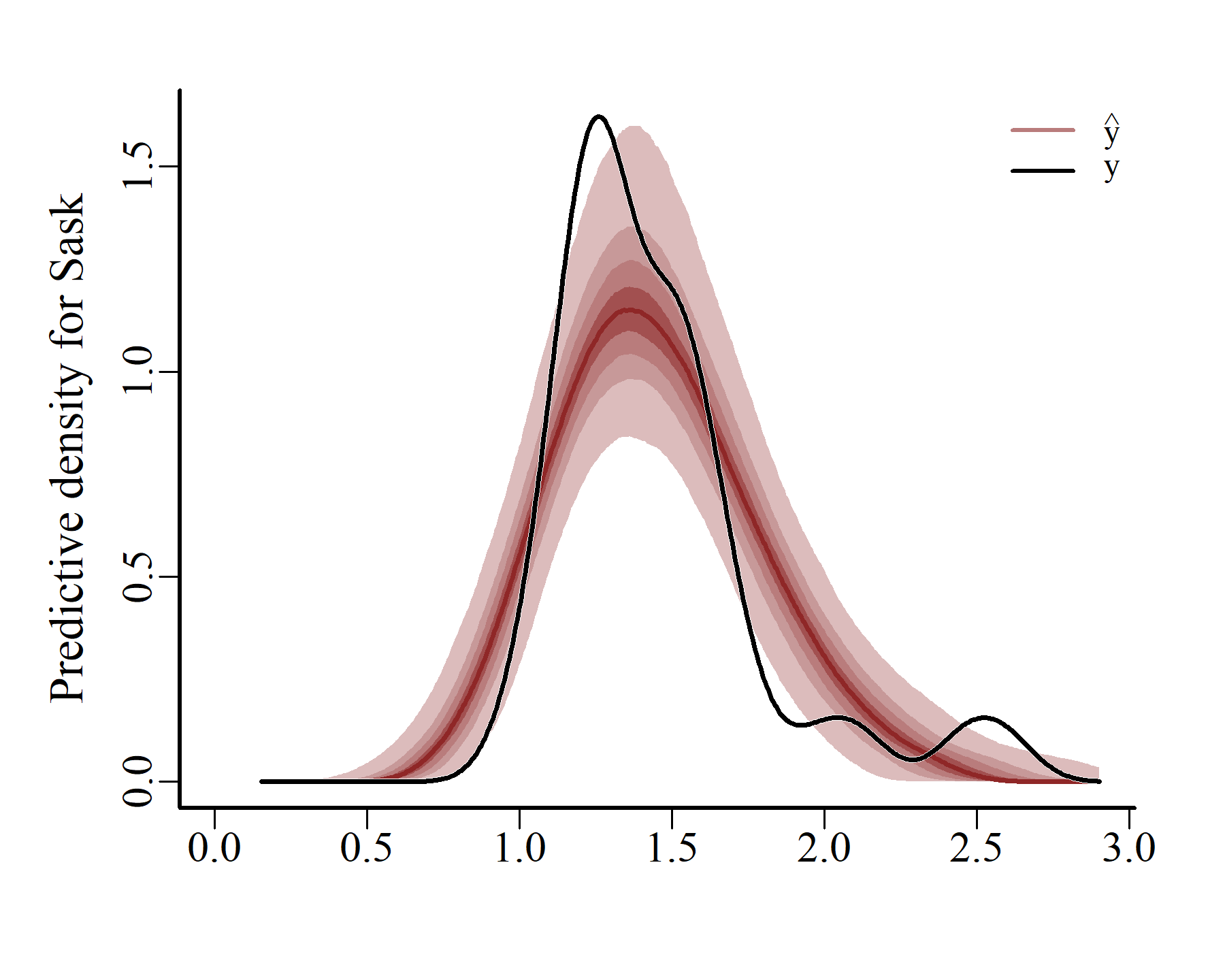
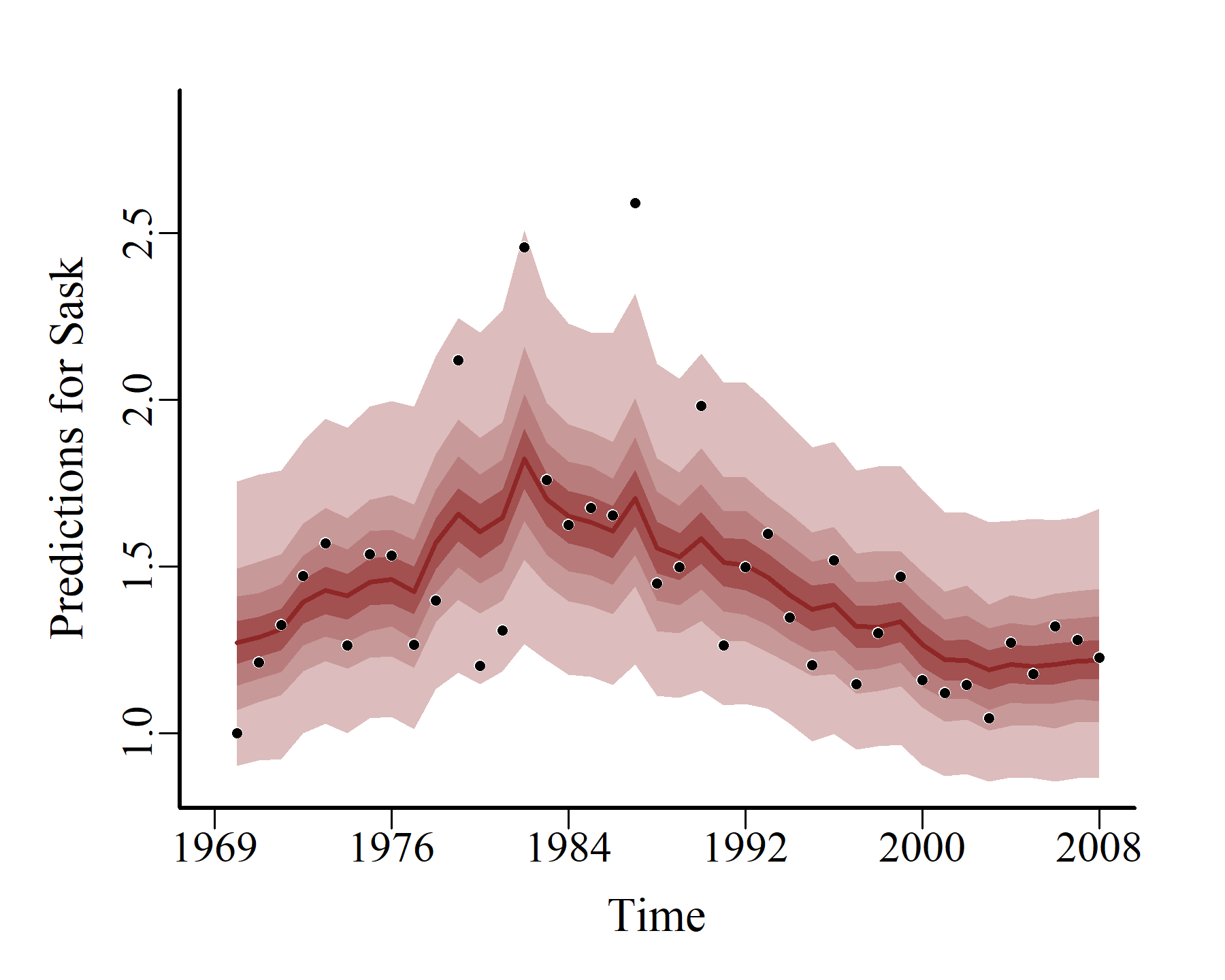
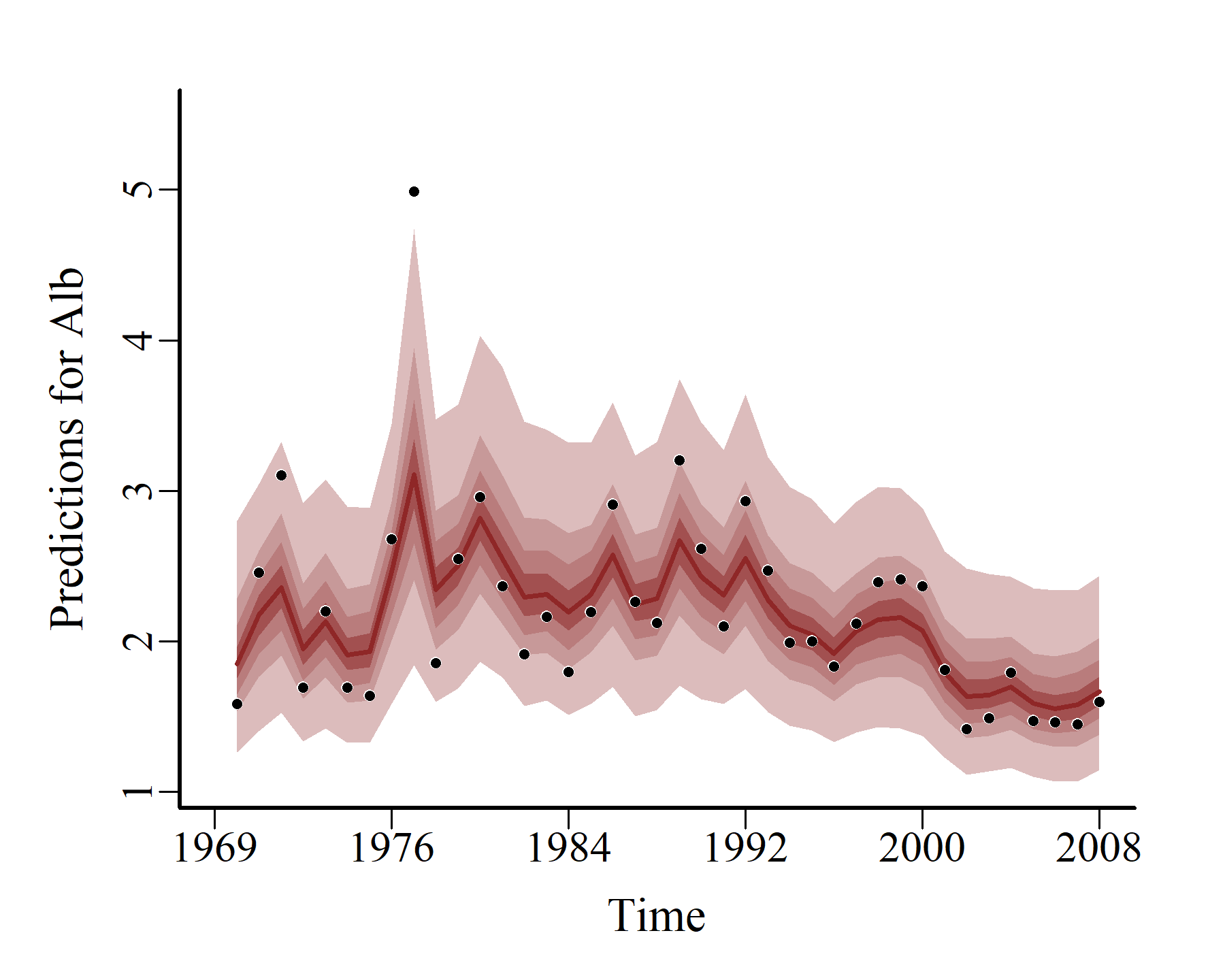
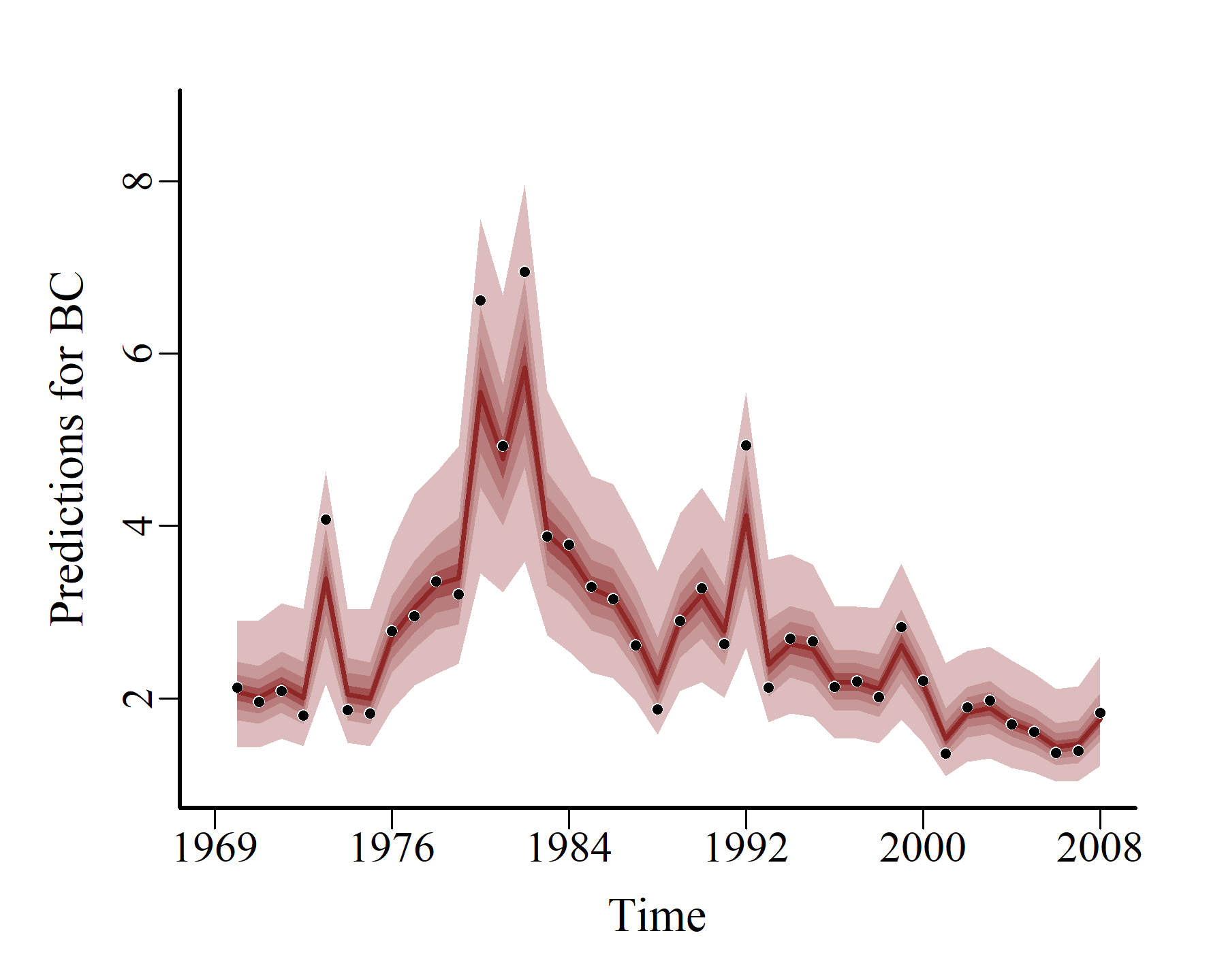
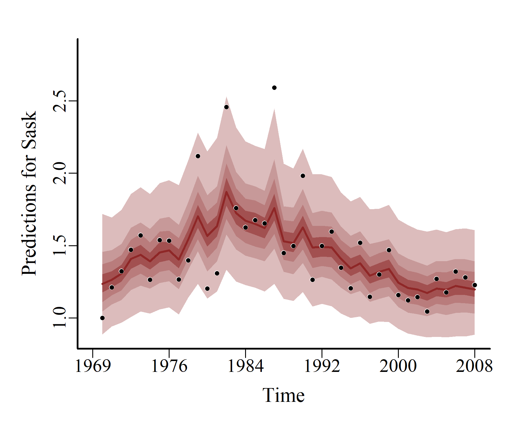
These plots match the data more closely, which is expected when using a flexible autoregressive process to capture the unobserved dynamics. Next we can compute and plot probabilistic conditional hindcasts for each series:

hcs <- hindcast(varmod)

plot(hcs,
     series = 1)

plot(hcs,
     series = 2)

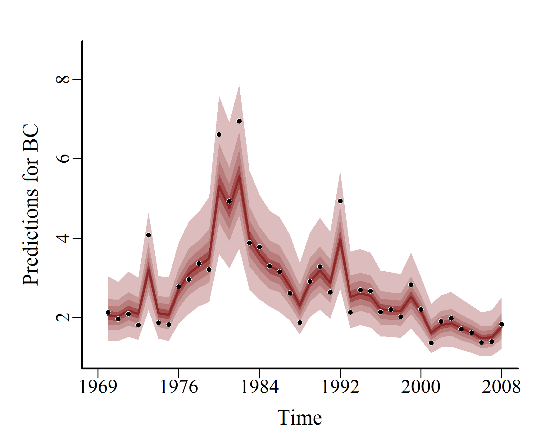
plot(hcs,
     series = 3)

Model expansion

Given the subtle variations in the shapes of these observed distributions for each series, there may be support for fitting an equivalent model that allows the Gamma shape parameters to vary among series. Let’s fit a second model that allows this:

varmod2 <- mvgam(
    # Observation formula, empty to only consider the Gamma observation process
  formula = adj_count ~ -1,
  
  # Process model formula that includes regional intercepts 
  trend_formula = ~ region,
  
  # A VAR(1) dynamic process with fully parameterized covariance matrix Sigma
  trend_model = VAR(cor = TRUE),
  
  # Modified prior distributions using brms::prior()
  priors = c(prior(std_normal(), class = Intercept_trend),
             prior(std_normal(), class = b),
             prior(exponential(2.5), class = sigma)),
  
  # The time series data in 'long' format
  data = model_data,
  
  # A Gamma observation family
  family = Gamma(),
  
  # Varying Gamma shape parameters per series
  share_obs_params = FALSE,
  
  # Stan control arguments
  adapt_delta = 0.95,
  burnin = 1000,
  samples = 1000,
  silent = 2
)

This model also fits well and encounters few sampling issues

summary(varmod2)

## GAM observation formula:
## adj_count ~ 1
## 
## GAM process formula:
## ~region
## 
## Family:
## Gamma
## 
## Link function:
## log
## 
## Trend model:
## VAR(cor = TRUE)
## 
## N process models:
## 3 
## 
## N series:
## 3 
## 
## N timepoints:
## 40 
## 
## Status:
## Fitted using Stan 
## 4 chains, each with iter = 2000; warmup = 1000; thin = 1 
## Total post-warmup draws = 4000
## 
## 
## Observation shape parameter estimates:
##          2.5% 50% 97.5% Rhat n_eff
## shape[1]   12  26   130 1.01   350
## shape[2]   13  40   220 1.01   349
## shape[3]   21  39   120 1.02   159
## 
## GAM observation model coefficient (beta) estimates:
##             2.5% 50% 97.5% Rhat n_eff
## (Intercept)    0   0     0  NaN   NaN
## 
## Process model VAR parameter estimates:
##          2.5%    50% 97.5% Rhat n_eff
## A[1,1] -0.032  0.560  1.00 1.01   731
## A[1,2] -0.400 -0.016  0.27 1.00  1349
## A[1,3] -0.073  0.450  1.70 1.00   514
## A[2,1] -0.310  0.400  2.80 1.02   199
## A[2,2] -0.580  0.340  0.83 1.01   462
## A[2,3] -0.290  0.640  2.70 1.00   530
## A[3,1] -0.075  0.170  1.30 1.01   150
## A[3,2] -0.250  0.034  0.26 1.01   585
## A[3,3]  0.012  0.570  0.97 1.00   527
## 
## Process error parameter estimates:
##               2.5%      50%  97.5% Rhat n_eff
## Sigma[1,1]  0.0018  0.01800 0.0620 1.03   159
## Sigma[1,2] -0.0076  0.00840 0.0340 1.00   898
## Sigma[1,3] -0.0120 -0.00054 0.0076 1.00   912
## Sigma[2,1] -0.0076  0.00840 0.0340 1.00   898
## Sigma[2,2]  0.0180  0.05400 0.1200 1.01   566
## Sigma[2,3] -0.0078  0.00420 0.0200 1.00  1594
## Sigma[3,1] -0.0120 -0.00054 0.0076 1.00   912
## Sigma[3,2] -0.0078  0.00420 0.0200 1.00  1594
## Sigma[3,3]  0.0013  0.00720 0.0300 1.01   292
## 
## GAM process model coefficient (beta) estimates:
##                    2.5%   50% 97.5% Rhat n_eff
## (Intercept)_trend  0.39  0.72  0.95    1  1272
## regionBC_trend    -0.13  0.14  0.36    1  1581
## regionSask_trend  -0.55 -0.40 -0.21    1   892
## 
## Stan MCMC diagnostics:
## n_eff / iter looks reasonable for all parameters
## Rhats above 1.05 found for 1 parameters
##  *Diagnose further to investigate why the chains have not mixed
## 11 of 4000 iterations ended with a divergence (0.275%)
##  *Try running with larger adapt_delta to remove the divergences
## 0 of 4000 iterations saturated the maximum tree depth of 12 (0%)
## E-FMI indicated no pathological behavior
## 
## Samples were drawn using NUTS(diag_e) at Fri Sep 27 12:58:12 PM 2024.
## For each parameter, n_eff is a crude measure of effective sample size,
## and Rhat is the potential scale reduction factor on split MCMC chains
## (at convergence, Rhat = 1)

But now we have three shape parameters to inspect:

mcmc_plot(varmod2,
          variable = 'shape',
          regex = TRUE,
          type = 'trace')

The unconditional posterior predictive checks look slightly better for the first and third series ('Alb' and 'Sask’):

pp_check(varmod2,
         type = "dens_overlay_grouped",
         group = "region",
         ndraws = 50)

And so do the probabilistic conditional hindcasts:

hcs <- hindcast(varmod2)

plot(hcs,
     series = 1)

plot(hcs,
     series = 2)

plot(hcs,
     series = 3)

Model comparison with `loo_compare()`

The plots for the second model look slightly better for some of the series, but of course this is a more complex model so we may expect that. Generally we may want to select among these two competing models, and the approximate leave-one-out cross-validation routines provided by the loo package allow us to do this. We simply call loo_compare() and feed in the set of models that we’d like to compare:

loo_compare(varmod, varmod2)

##         elpd_diff se_diff
## varmod2       0.0     0.0
## varmod       -3.6     1.9

The second model has slightly but consistently higher leave-one-out expected log predictive densities than the first model, so it appears to be slightly favoured. But of course we may wish to use other forms of model comparison, such as computing proper scoring rules for out-of-sample probabilistic forecasts. But for simplicity we will stick with the second model for further interrogation.

Interrogating VAR(1) models in `mvgam`

There are many useful questions that can be approached using VAR models, which I eluded to at the beginning of this post. mvgam has support for a growing number of investigations that can be performed using built-in functions, and this section will highlight some of those functionalities.

Inspecting AR coefficient and covariance estimates

One of the first things we might want to do with a VAR(1) model is to inspect the $A$ matrix, which includes the autoregressive coefficients that estimate lagged dependence and cross-dependence between the elements of the latent process model. By default bayesplot will plot these in the wrong order, so a bit of rearranging of the parameter estimates is needed to show the full matrix of estimates:

A_pars <- matrix(NA, nrow = 3, ncol = 3)
for(i in 1:3){
  for(j in 1:3){
    A_pars[i, j] <- paste0('A[', i, ',', j, ']')
  }
}
mcmc_plot(varmod2,
          variable = as.vector(t(A_pars)),
          type = 'hist') +
  geom_vline(xintercept = 0,
             col = 'white',
             linewidth = 2) +
  geom_vline(xintercept = 0,
             linewidth = 1)

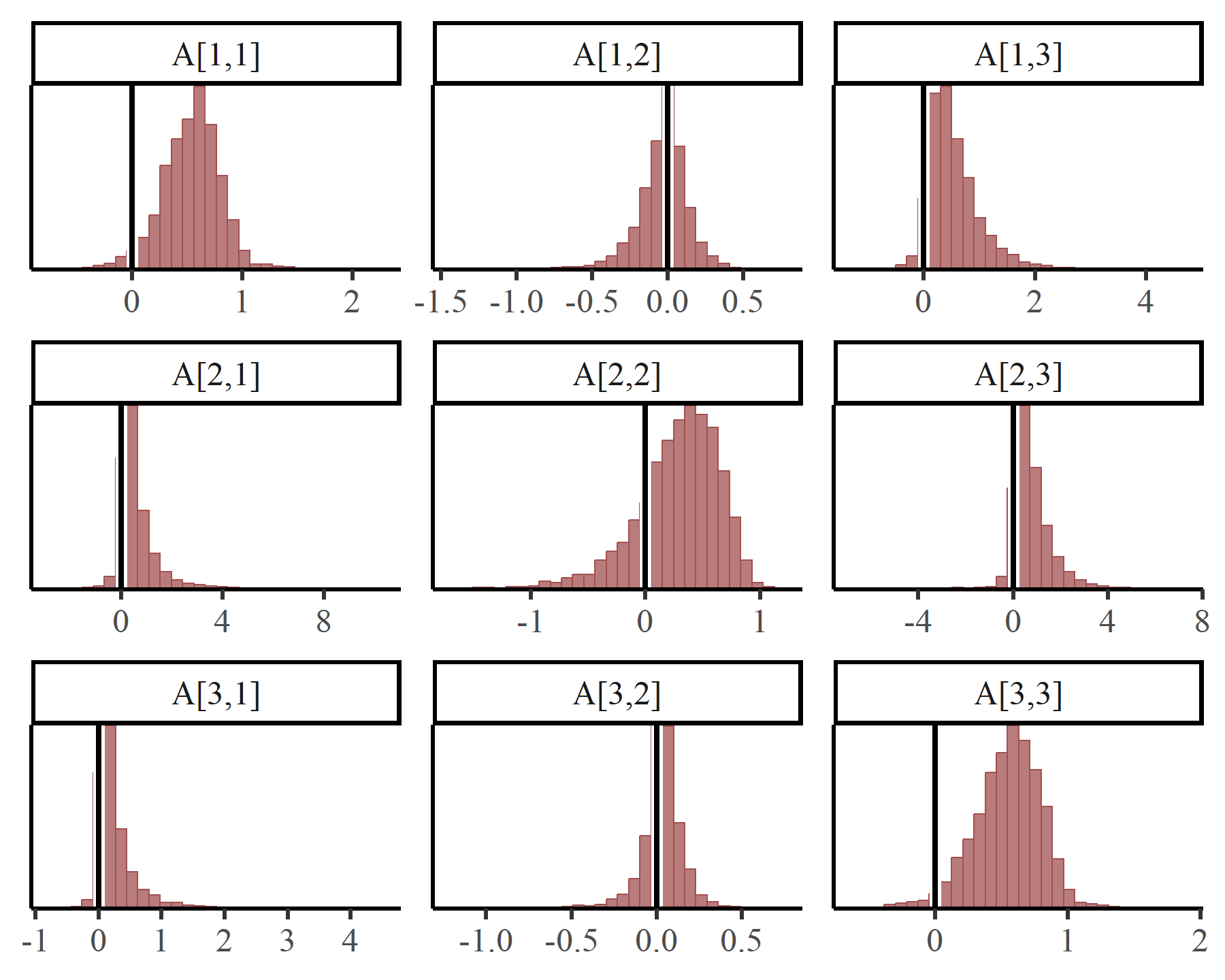
mvgam vector autoregressive coefficient inspection

This plot makes it clear that there is broad posterior support for positive interactions among the three latent processes. For example, the estimates in A[2,3] capture how an increase in the process for series 2 ('BC') at time $t$ is expected to impact the process for series 3 ('Sask') at time $t+1$. This might make biological sense as it could be possible that increasing populations in one region lead to subsequent increases in other regions due to dispersal events.

We might also want to look at evidence for contemporaneous associations among these processes, which are captured in the covariance matrix $\Sigma_{process}$. The same rearrangement of parameters is needed to get these in the right order:

Sigma_pars <- matrix(NA, nrow = 3, ncol = 3)
for(i in 1:3){
  for(j in 1:3){
    Sigma_pars[i, j] <- paste0('Sigma[', i, ',', j, ']')
  }
}
mcmc_plot(varmod2,
          variable = as.vector(t(Sigma_pars)),
          type = 'hist') +
  geom_vline(xintercept = 0,
             col = 'white',
             linewidth = 2) +
  geom_vline(xintercept = 0,
             linewidth = 1)

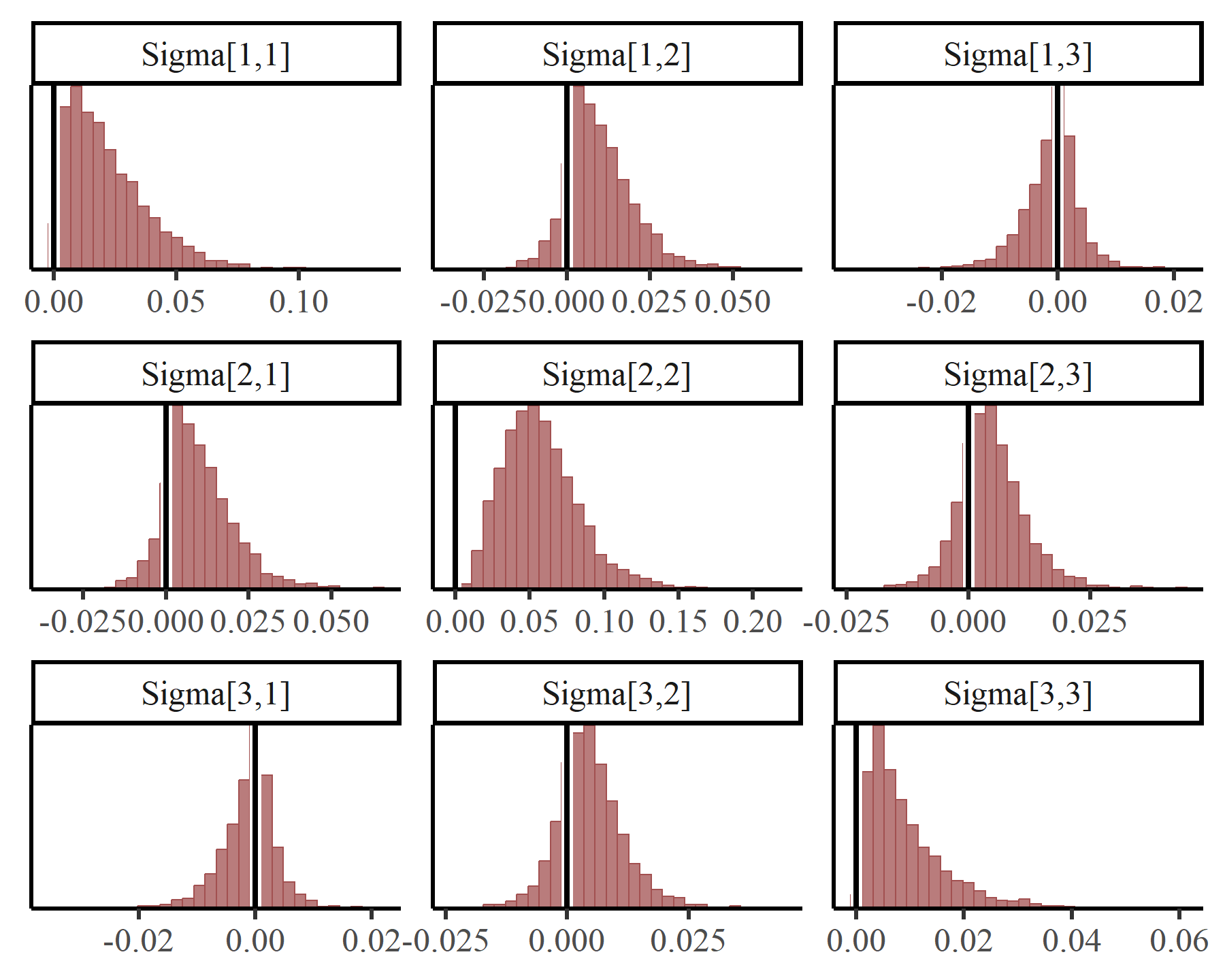
mvgam vector autoregressive covariance inspection

Again we see many positive covariances which suggests that these processes are not evolving independently, but are rather likely to be co-responding to some broader phenomena

Impulse Response Functions

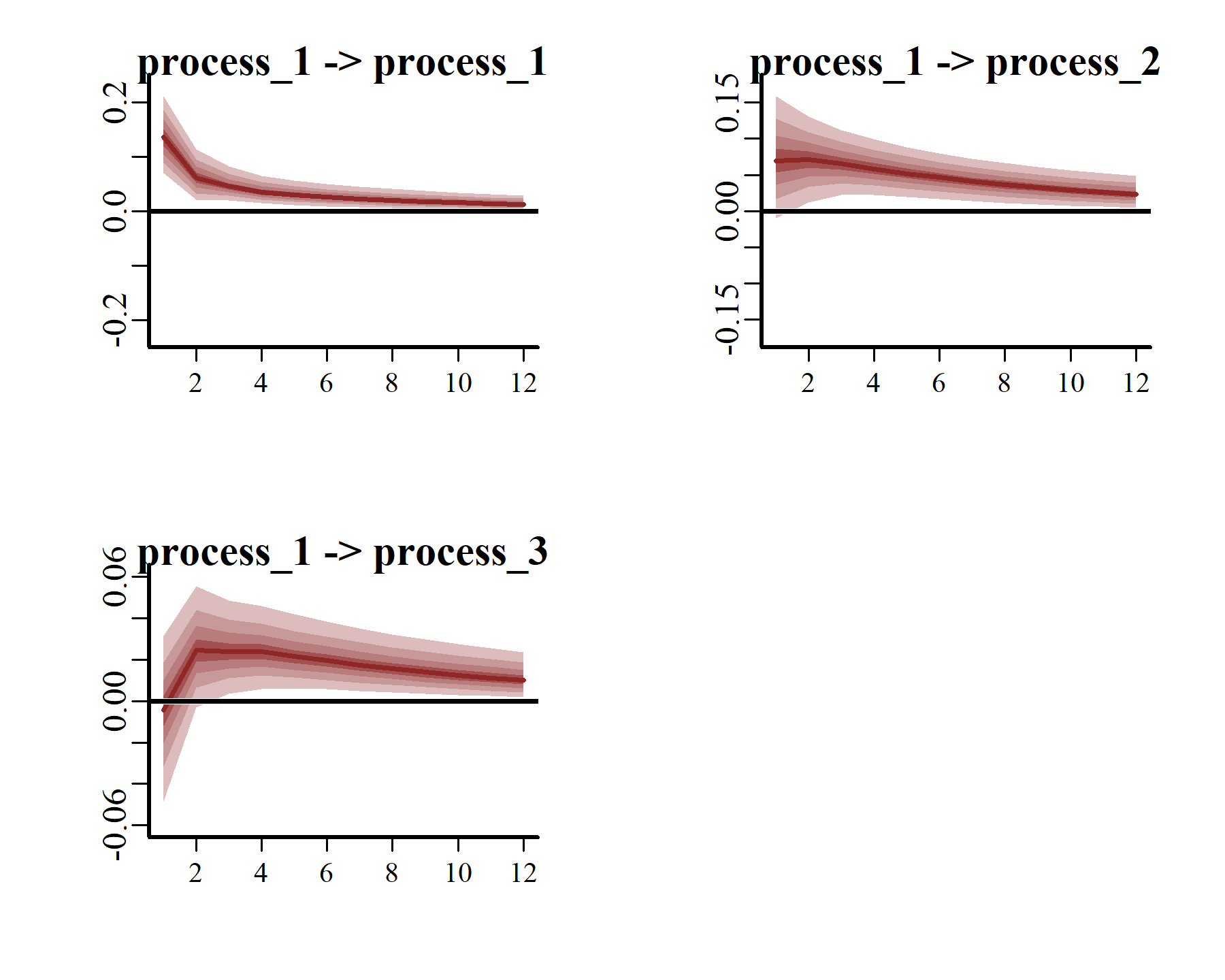
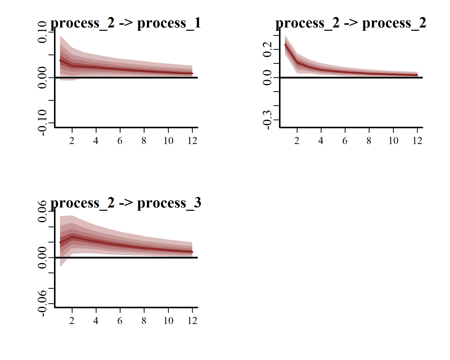
Generalized or Orthogonalized Impulse Response Functions (IRFs) can be computed using the posterior estimates of Vector Autoregressive parameters from mvgam models fitted with VAR() trend models. This function runs a simulation whereby a positive “shock” is generated for a target process at time $t = 0$. All else remaining stable, it then monitors how each of the remaining processes in the latent VAR would be expected to respond over the forecast horizon $h$. The function computes IRFs for all processes in the object and returns them in an array that can be plotted using the S3 plot() function. Here we will use the generalized IRF, which makes no assumptions about the order in which the series appear in the VAR process, and inspect how each process is expected to respond to a sudden, positive pulse from the other processes over a horizon of 12 years.

irfs <- irf(varmod2,
            h = 12,
            orthogonal = FALSE)

plot(irfs,
     series = 1)

mvgam vector autoregressive impulse response functions

plot(irfs,
     series = 2)

plot(irfs,
     series = 3)

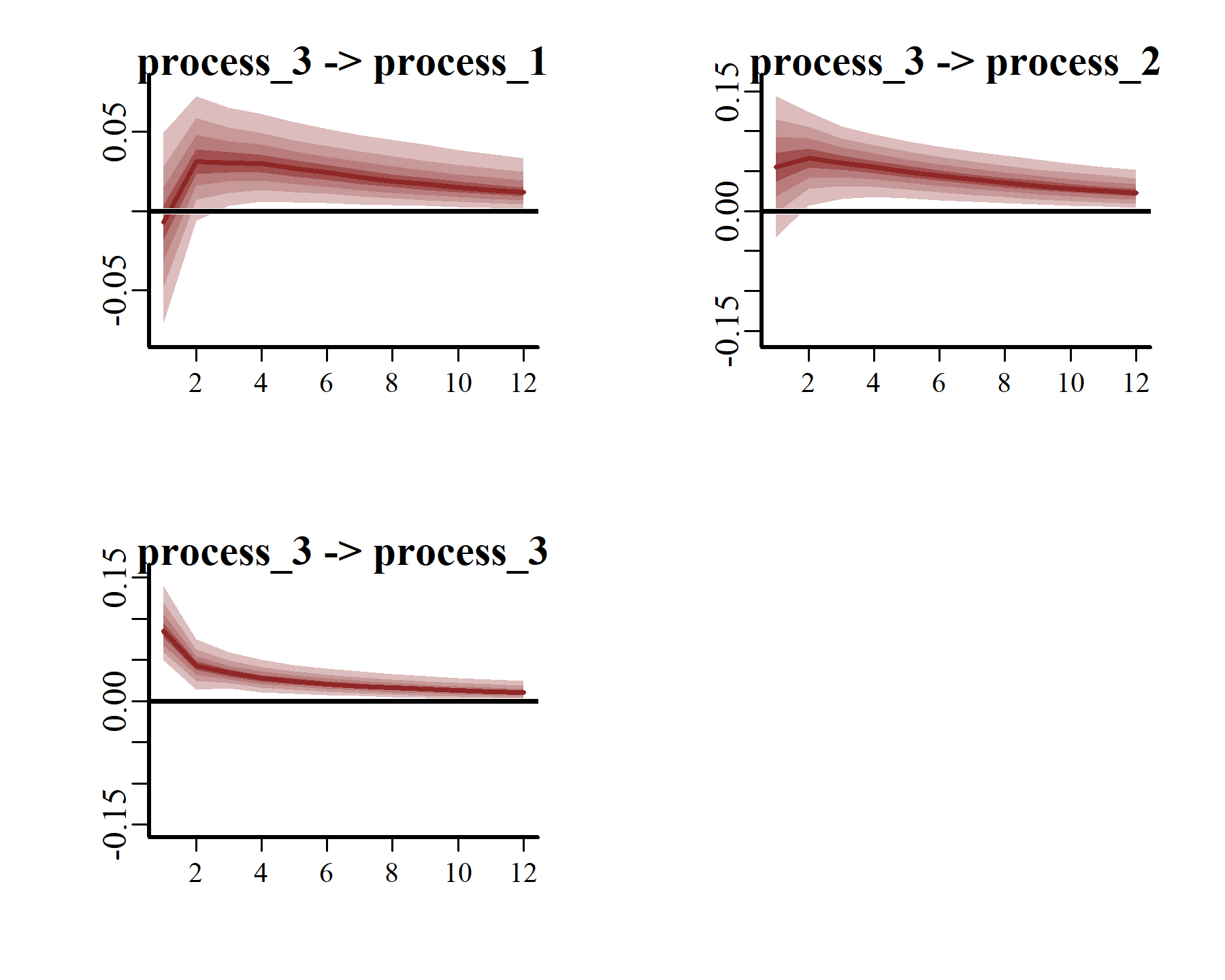
These plots make it clear that, if one region experienced a temporary pulse in the number of American kestrels, we’d expect the remaining regions to show contemporaneous and/or subsequent increases over the following years. Moreover, we’d expect the effects of this pulse to reverberate for many years, thanks to the strong positive dependencies that are shown among all three series.

Forecast Error Variance Decompositions

Using the same logic as above, we can inspect forecast error variance decompositions (FEVDs) for each process using the fevd() function. This type of analysis asks how orthogonal shocks to all process in the system contribute to the variance of forecast uncertainty for a focal process over increasing horizons. In other words, the proportion of the forecast variance of each latent time series can be attributed to the effects of the other series in the VAR proces. FEVDs are useful because some shocks may not be expected to cause variations in the short-term but may cause longer-term fluctuations

fevds <- fevd(varmod2, h = 12)

The S3 plot() function for these objects returns a ggplot object that shows the mean expected contribution to forecast error variance for each process in the VAR model:

plot(fevds) +
  scale_fill_manual(values = c("#DCBCBC",
                               "#A25050",
                               "#5C0000"))

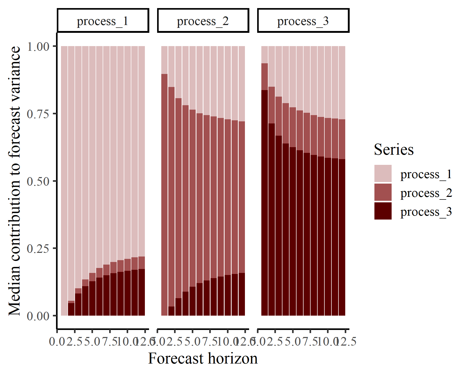
mvgam vector autoregressive forecast error variance decompositions

This plot shows that the variance of forecast uncertainty for each process is initially dominated by contributions from that same process (i.e. self-dependent effects) but that effects from other processes become more important over increasing forecast horizons. Given what we saw from the IRF plots above, these long-term contributions from interactions among the processes makes sense.

Community stability metrics

mvgam can also calculate a range of community stability metrics, which can be used to assess how important inter-series dependencies are to the variability of a multivariate system and to ask how systems are expected to respond to environmental perturbations. The stability() function computes a posterior distribution for the long-term stationary forecast distribution of the system, which has mean $\mu_{\infty}$ and variance $\Sigma_{\infty}$, to then calculate the following quantities:

prop_int: Proportion of the volume of the stationary forecast distribution that is attributable to lagged interactions (i.e. how important are the autoregressive interaction coefficients in $A$ for explaining the shape of the stationary forecast distribution?): $det(A)^2$
prop_int_adj: Same as prop_int but scaled by the number of series $p$ to facilitate direct comparisons among systems with different numbers of interacting variables: $det(A)^{2/p}$
prop_int_offdiag: Sensitivity of prop_int to inter-series interactions (i.e. how important are the off-diagonals of the autoregressive coefficient matrix $A$ for shaping prop_int?), calculated as the relative magnitude of the off-diagonals in the partial derivative matrix: $[2~det(A) (A^{-1})^T]$
prop_int_diag: Sensitivity of prop_int to intra-series interactions (i.e. how important are the diagonals of the autoregressive coefficient matrix $A$ for shaping prop_int?), calculated as the relative magnitude of the diagonals in the partial derivative matrix: $[2~det(A) (A^{-1})^T]$
prop_cov_offdiag: Sensitivity of $\Sigma_{\infty}$ to inter-series error correlations (i.e. how important are off-diagonal covariances in $\Sigma$ for shaping $\Sigma_{\infty}$?), calculated as the relative magnitude of the off-diagonals in the partial derivative matrix: $[2~det(\Sigma_{\infty}) (\Sigma_{\infty}^{-1})^T]$
prop_cov_diag: Sensitivity of $\Sigma_{\infty}$ to error variances (i.e. how important are diagonal variances in $\Sigma$ for shaping $\Sigma_{\infty}$?), calculated as the relative magnitude of the diagonals in the partial derivative matrix: $[2~det(\Sigma_{\infty}) (\Sigma_{\infty}^{-1})^T]$
reactivity: A measure of the degree to which the system moves away from a stable equilibrium following a perturbation. Values > 0 suggest the system is reactive, whereby a perturbation of the system in one period can be amplified into the next period. If $\sigma_{max}(A)$ is the largest singular value of $A$, then reactivity is defined as: $log\sigma_{max}(A)$
mean_return_rate: Asymptotic (long-term) return rate of the mean of the transition distribution to the stationary mean, calculated using the largest eigenvalue of the matrix $A$: $max(\lambda_{A})$. Lower values suggest greater stability of the system
var_return_rate: Asymptotic (long-term) return rate of the variance of the transition distribution to the stationary variance: $max(\lambda_{A \otimes{A}})$. Again, lower values suggest greater stability of the system

metrics <- stability(varmod2)

We can plot the posterior distribution of reactivity, which is perhaps the most commonly calculated metric of ecological community stability, using ggplot():

ggplot(metrics, aes(x = reactivity)) +
  myhist() +
  labs(x = 'Reactivity', y = '') +
  geom_vline(xintercept = 0, col = 'white', linewidth = 2.5) +
  geom_vline(xintercept = 0, linewidth = 1.5) +
  hist_theme()

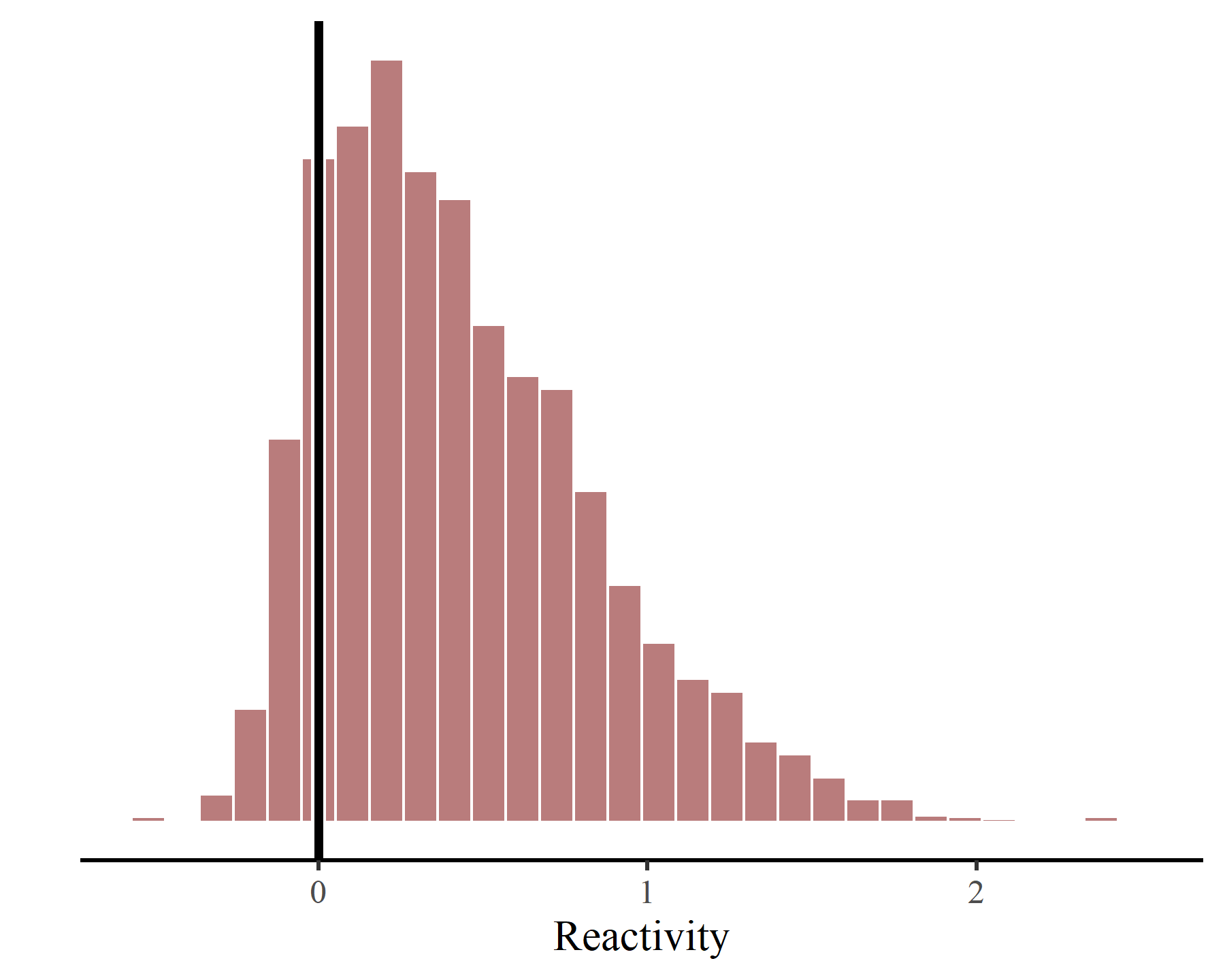
mvgam vector autoregressive community reactivity estimates

This system is considered to be “reactive”, whereby this index of the community’s short-term response to perturbations is mostly estimated to be >0. Again this is not surprising, as both the irf() and fevd() plots show that the time series of adjusted counts in each region is highly dependent on time-lagged adjusted counts in other regions.

Another useful question to ask from these metrics is what are the relative importances of the diagonals for determining the contributions of the $A$ and $\Sigma$ matrices to the shape of the stationary forecast distribution. In other words, we can decompose the contributions of these two matrices to the system’s stochastic equilibrium to understand which components (i.e. the self-dependence vs the inter-dependence effects) seem to have the biggest influences on the variability of the system. What follows is some rather long-winded code that will calculate and plot these contributions, using some helpful example code provided by Matthew Kay, maintainer of the tidybayes package

# Gather posterior estimates of relative contributions for each matrix
# into a tidy format for tidybayes plotting
prop_df <- rbind(metrics %>%
    dplyr::select(prop_cov_diag,
                  prop_cov_offdiag) %>%
    dplyr::rename(diagonals = prop_cov_diag,
                  off_diagonals = prop_cov_offdiag) %>%
    dplyr::mutate(.draw = 1:dplyr::n(),
                  group = 'Process error (Sigma)') %>%
    tidyr::pivot_longer(c(diagonals, off_diagonals),
                        names_to = 'Parameters',
                        values_to = 'proportion'),
  metrics %>%
    dplyr::select(prop_int_diag,
                  prop_int_offdiag) %>%
    dplyr::rename(diagonals = prop_int_diag,
                  off_diagonals = prop_int_offdiag) %>%
    dplyr::mutate(.draw = 1:dplyr::n(),
                  group = 'Autoregressive coefs (A)') %>%
    tidyr::pivot_longer(c(diagonals, off_diagonals),
                        names_to = 'Parameters',
                        values_to = 'proportion'))

# Calculate blurred color maps to graphically represent uncertainty
# in these contributions
p <- seq(0, 1 - .Machine$double.eps, length.out = 200)
df_curves <- prop_df %>%
  dplyr::mutate(cumulative_proportion = cumsum(proportion),
                .by = c(.draw, group)) |>
  dplyr::reframe(
    `P(value)` = (1 - ecdf(cumulative_proportion)(p)) *
      ecdf(cumulative_proportion - proportion)(p),
    proportion = p,
    .by = c(group, Parameters))

# Set the colours and their labels
fill_scale <- scale_fill_manual(values = c("lightgrey", "#A25050"))
fill_scale$train(c("diagonals", "off_diagonals"))

Now we can plot these relative contributions in a way that aims to represent their associated posterior uncertainties

df_curves %>%
  summarise(color = encode_colour(`P(value)` %*%
                            decode_colour(fill_scale$map(Parameters),
                                          to = "oklab"),
                          from = "oklab"),
    .by = c(group,
            proportion)) %>%
  ggplot() +
  geom_blank(aes(fill = Parameters),
             data = data.frame(Parameters = c("diagonals",
                                              "off_diagonals"))) +
  geom_slab(aes(y = proportion,
                x = group,
                fill = I(color),
                group = NA),
    thickness = 1,
    fill_type = "auto",
    side = "both") +
  stat_pointinterval(
    aes(x = group,
        y = proportion,
        group = Parameters),
    data = prop_df |>
      mutate(proportion = cumsum(proportion),
             .by = c(.draw, group)) |>
      filter(Parameters != "off_diagonals")) +
  fill_scale +
  scale_y_continuous(limits = c(0, 1)) +
  coord_cartesian(expand = FALSE) +
  labs(x = '',
       y = 'Contribution to stationary distribution')

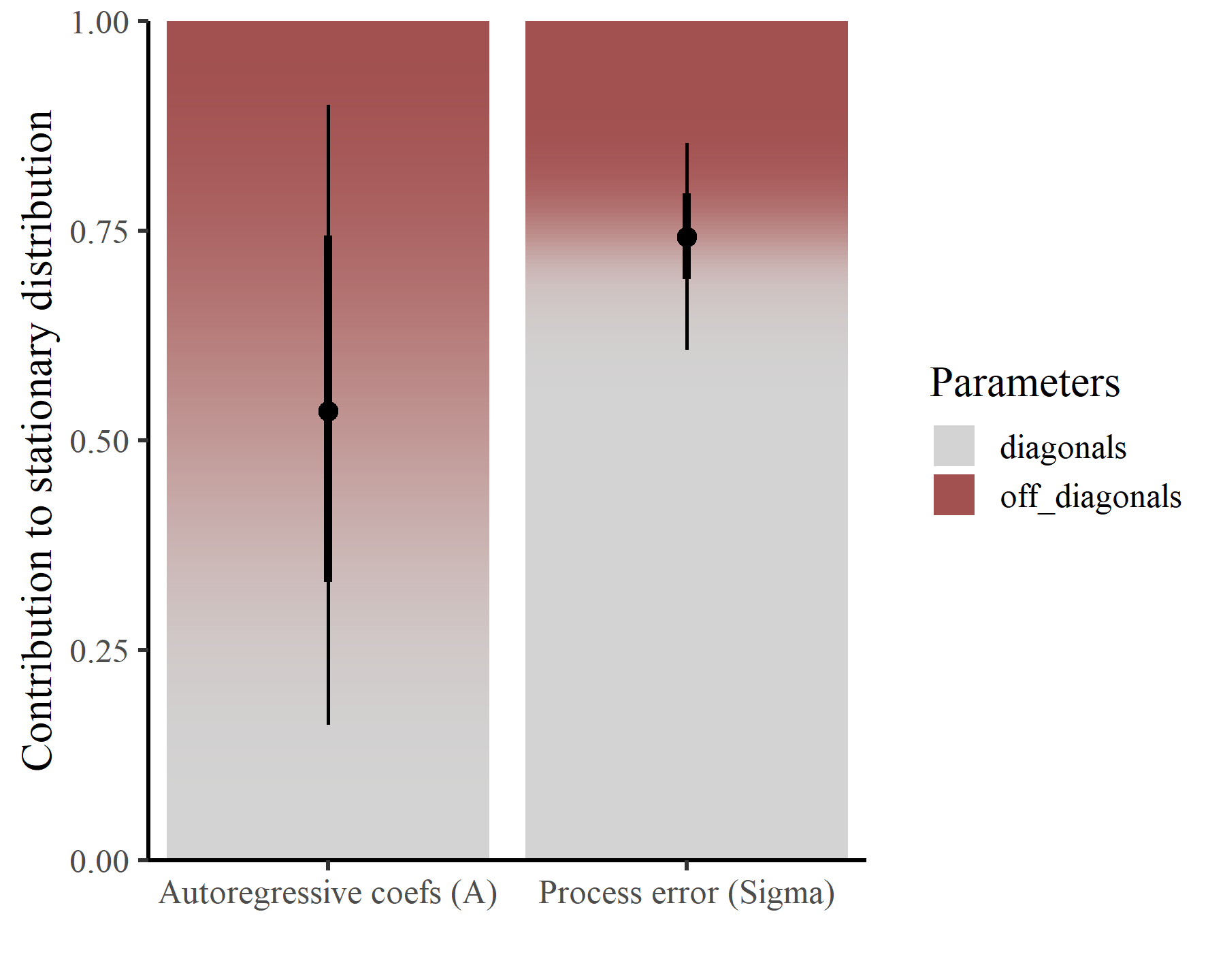
And there we have it. This plot demonstrates that, within the contribution of the $A$ matrix to the stable distribution, the off-diagonals (i.e. the lagged autoregressive interaction effects) play a sizable role. However, within the contribution of the $\Sigma$ matrix to the stable distribution, the diagonals (i.e. the process variances) are much more important than are the off-diagonal covariances. This gives us some insights into the relative importances of lagged vs contemporaneous “interactions” and can hopefully facilitate more in-depth ecological analyses.

Also, although we haven’t covered it in this example, there is of course no reason why you cannot include complex covariate effects in either the process or observation models. Indeed, mvgam() can readily handle a wide range of effects including multidimensional penalized smooth functions, Gaussian Process functions, monotonic smooth functions, distributed lag nonlinear effects, seasonality and time-varying seasonality, and hierarchical effects. It is also easy to generate probabilistic forecasts from these models, which you can learn more about by reading the forecast and forecast evaluation vignette. These options should hopefully make mvgam a very attractive resource for tackling real-world multivariate time series when we do not wish to ignore important drivers or use time series transformations that make both inference and prediction difficult. Thanks for your time!