First release of mvgam(v1.1.0) to CRAN
By Nicholas Clark in rstats package mvgam
May 8, 2024
Welcoming mvgam to the Comprehensive R Archive Network (CRAN)
The goal of mvgam is to use a Bayesian framework to estimate parameters of Dynamic Generalized Additive Models (DGAMs) for time series with dynamic trend components. The package provides an interface to fit Bayesian DGAMs using
Stan as the backend, and is particularly suited to the estimation of complex State-Space models. The formula syntax is based on that of the package
mgcv to provide a familiar GAM modelling interface. There is also built-in support for the increasingly powerful
marginaleffects package to make interpretation easy. The motivation for the package and some of its primary objectives are described in detail by Clark & Wells 2022 (published in
Methods in Ecology and Evolution). An introduction to the package and some worked examples are also shown in the below seminar:
Ecological Forecasting with Dynamic Generalized Additive Models DGAMs)
The first release of mvgam
has now been published on CRAN. While the package has featured on this blog before, for example when I explained
hierarchical distributed lag models and
how to model temporally autocorrelated time series with nonlinear trends, I have not thorougly introduced the it yet. So the purpose of this brief post is to cover some of the features of this stable release, and to hint at a few of the development goals for upcoming releases.
What are Generalized Additive Models (GAMs)?
Generalized Additive Models (GAMs) are flexible tools that replace one or more predictors in a Generalized Linear Model (GLM) with smooth functions of predictors. These are helpful for learning arbitrarily complex, nonlinear relationships between predictors and conditional responses without needing a priori expectations about the shapes of these relationships. Rather, they are learned using penalized smoothing splines.
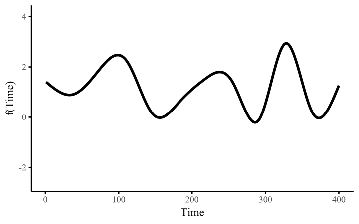
How do these work? The secret is a basis expansion, which in lay terms means that the covariate (time, in this example) is evaluated at a smaller set of basis functions designed to cover the range of the observed covariate values. Below is one particular type of basis, called a cubic regression basis.

Each basis function acts on its own local neighbourhood of the covariate. Once we have constructed the basis, we can estimate weights for each function. The weights allow the basis functions to have different impacts on the shape of the spline. They also give us a target for learning splines from data, as the weights act as the regression coefficients.
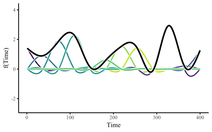
There are many more types of basis expansions that can be used to form penalized smooths, including multidimensional smooths, spatial smooths or even monotonic smooths. For more information on GAMs and how they can smooth through data, see my blogpost on how to interpret nonlinear effects from Generalized Additive Models.
What does mvgam do?
mvgam is designed to propagate unobserved temporal processes to capture latent dynamics in the observed time series. This works in a state-space format, with the temporal trend evolving independently of the observation process. Briefly, assume \(\tilde{\boldsymbol{y}}_{i,t}\) is the conditional expectation of response variable \(\boldsymbol{i}\) at time \(\boldsymbol{t}\). Assuming \(\boldsymbol{y_i}\) is drawn from an exponential distribution with an invertible link function, the linear predictor for a multivariate Dynamic GAM can be written as:
$$for~i~in~1:N_{series}~...$$
$$for~t~in~1:N_{timepoints}~...$$
$$g^{-1}(\tilde{\boldsymbol{y}}_{i,t})=\alpha_{i}+\sum\limits_{j=1}^J\boldsymbol{s}_{i,j,t}\boldsymbol{x}_{j,t}+\boldsymbol{z}_{i,t}\,,$$
Here \(\alpha\) are the unknown intercepts, the \(\boldsymbol{s}\)’s are unknown smooth functions of covariates \((\boldsymbol{x})\)’s, which can potentially vary among the response series, and \(\boldsymbol{z}\) are dynamic latent processes. Each smooth function \(\boldsymbol{s_j}\) is composed of basis expansions whose coefficients, which must be estimated, control the functional relationship between \(\boldsymbol{x}_{j}\) and \(g^{-1}(\tilde{\boldsymbol{y}})\). But note that we can also include smooth functions of covariates in the process models \(\boldsymbol{z}\).
Several advantages of GAMs are that they can model a diversity of response families, including discrete distributions (i.e. Poisson, Negative Binomial, Gamma) that accommodate common ecological features such as zero-inflation or overdispersion, and that they can be formulated to include hierarchical smoothing for multivariate responses. mvgam supports a number of different observation families, which are summarized below.
Supported observation families
mvgam was originally designed to analyse and forecast time series of non-negative integer-valued data (counts). These data are traditionally challenging to analyse with existing time series analysis packages. But further development of mvgam has resulted in support for a growing number of observation families that extend to other types of data. Currently, the package can handle data for the following families:
| Distribution | Function | Support | Extra parameter(s) |
|---|---|---|---|
| Gaussian (identity link) | gaussian() |
Real values in \((-\infty, \infty)\) |
\(\sigma\) |
| Student’s T (identity link) | student-t() |
Heavy-tailed real values in \((-\infty, \infty)\) |
\(\sigma\), \(\nu\) |
| LogNormal (identity link) | lognormal() |
Positive real values in \([0, \infty)\) |
\(\sigma\) |
| Gamma (log link) | Gamma() |
Positive real values in \([0, \infty)\) |
\(\alpha\) |
| Beta (logit link) | betar() |
Real values (proportional) in \([0,1]\) |
\(\phi\) |
| Bernoulli (logit link) | bernoulli() |
Binary data in \({0,1}\) |
- |
| Poisson (log link) | poisson() |
Non-negative integers in \((0,1,2,...)\) |
- |
| Negative Binomial2 (log link) | nb() |
Non-negative integers in \((0,1,2,...)\) |
\(\phi\) |
| Binomial (logit link) | binomial() |
Non-negative integers in \((0,1,2,...)\) |
- |
| Beta-Binomial (logit link) | beta_binomial() |
Non-negative integers in \((0,1,2,...)\) |
\(\phi\) |
| Poisson Binomial N-mixture (log link) | nmix() |
Non-negative integers in \((0,1,2,...)\) |
- |
For all supported observation families, any extra parameters that need to be estimated (i.e. the \(\sigma\) in a Gaussian model or the \(\phi\) in a Negative Binomial model) are by default estimated independently for each series. However, users can opt to force all series to share extra observation parameters using share_obs_params = TRUE in mvgam(). Note that default link functions cannot currently be changed.
Supported temporal dynamic processes
The dynamic processes that mvgam can fit to time series can take a wide variety of forms, some of which can be multivariate to allow the different time series to interact or be correlated. When using the mvgam() function, the user chooses between different process models with the trend_model argument. Available process models are described in
?mvgam_trends and detailed below.
Independent Random Walks
Use trend_model = 'RW' or trend_model = RW() to set up a model where each series in data has independent latent temporal dynamics of the form:
$$\begin{align*}
 z_{i,t} & \sim \text{Normal}(z_{i,t-1}, \sigma_i) \end{align*}$$
Process error parameters \(\sigma\) are modeled independently for each series. If a moving average process is required, use trend_model = RW(ma = TRUE) to set up the following:
$$\begin{align*}
 z_{i,t} & = z_{i,t-1} + \theta_i * error_{i,t-1} + error_{i,t} \\
 error_{i,t} & \sim \text{Normal}(0, \sigma_i) \end{align*}$$
Moving average coefficients \(\theta\) are independently estimated for each series and will be forced to be stationary by default \((abs(\theta)<1)\). Only moving averages of order \(q=1\) are currently allowed.
Multivariate Random Walks
If more than one series is included in data \((N_{series} > 1)\), a multivariate Random Walk can be set up using trend_model = RW(cor = TRUE), resulting in the following:
$$\begin{align*}
 z_{t} & \sim \text{MVNormal}(z_{t-1}, \Sigma) \end{align*}$$
Where the latent process estimate \(z_t\) now takes the form of a vector. The covariance matrix \(\Sigma\) will capture contemporaneously correlated process errors. It is parameterised using a Cholesky factorization, which requires priors on the series-level variances \(\sigma\) and on the strength of correlations using Stan’s lkj_corr_cholesky distribution.
Moving average terms can also be included for multivariate random walks, in which case the moving average coefficients \(\theta\) will be parameterised as an \(N_{series} * N_{series}\) matrix
Autoregressive processes
Autoregressive models up to \(p=3\), in which the autoregressive coefficients are estimated independently for each series, can be used by specifying trend_model = 'AR1', trend_model = 'AR2', trend_model = 'AR3', or trend_model = AR(p = 1, 2, or 3). For example, a univariate AR(1) model takes the form:
$$\begin{align*}
 z_{i,t} & \sim \text{Normal}(ar1_i * z_{i,t-1}, \sigma_i) \end{align*}$$
All options are the same as for Random Walks, but additional options will be available for placing priors on the autoregressive coefficients. By default, these coefficients will not be forced into stationarity, but users can impose this restriction by changing the upper and lower bounds on their priors. See ?get_mvgam_priors for more details.
Vector Autoregressive processes
A Vector Autoregression of order \(p=1\) can be specified if \(N_{series} > 1\) using trend_model = 'VAR1' or trend_model = VAR(). A VAR(1) model takes the form:
$$\begin{align*}
 z_{t} & \sim \text{Normal}(A * z_{t-1}, \Sigma) \end{align*}$$
Where \(A\) is an \(N_{series} * N_{series}\) matrix of autoregressive coefficients in which the diagonals capture lagged self-dependence (i.e. the effect of a process at time \(t\) on its own estimate at time \(t+1\)), while off-diagonals capture lagged cross-dependence (i.e. the effect of a process at time \(t\) on the process for another series at time \(t+1\)). By default, the covariance matrix \(\Sigma\) will assume no process error covariance by fixing the off-diagonals to \(0\). To allow for correlated errors, use trend_model = 'VAR1cor' or trend_model = VAR(cor = TRUE). A moving average of order \(q=1\) can also be included using trend_model = VAR(ma = TRUE, cor = TRUE).
Note that for all VAR models, stationarity of the process is enforced with a structured prior distribution that is described in detail in Heaps 2022
Heaps, Sarah E. “ Enforcing stationarity through the prior in vector autoregressions.” Journal of Computational and Graphical Statistics 32.1 (2023): 74-83.
Gaussian Processes
The final option for modelling temporal dynamics is to use a Gaussian Process with squared exponential kernel. These are set up independently for each series (there is currently no multivariate GP option), using trend_model = 'GP'. The dynamics for each latent process are modelled as:
$$\begin{align*}
 z & \sim \text{MVNormal}(0, \Sigma_{error}) \\
 \Sigma_{error}[t_i, t_j] & = \alpha^2 * exp(-0.5 * ((|t_i - t_j| / \rho))^2) \end{align*}$$
The latent dynamic process evolves from a complex, high-dimensional Multivariate Normal distribution which depends on \(\rho\) (often called the length scale parameter) to control how quickly the correlations between the model’s errors decay as a function of time. For these models, covariance decays exponentially fast with the squared distance (in time) between the observations. The functions also depend on a parameter \(\alpha\), which controls the marginal variability of the temporal function at all points; in other words it controls how much the GP term contributes to the linear predictor. mvgam capitalizes on some advances that allow GPs to be approximated using Hilbert space basis functions, which
considerably speed up computation at little cost to accuracy or prediction performance.
Piecewise logistic and linear trends
Modeling growth for many types of time series is often similar to modeling population growth in natural ecosystems, where there series exhibits nonlinear growth that saturates at some particular carrying capacity. The logistic trend model available in {mvgam} allows for a time-varying capacity \(C(t)\) as well as a non-constant growth rate. Changes in the base growth rate \(k\) are incorporated by explicitly defining changepoints throughout the training period where the growth rate is allowed to vary. The changepoint vector \(a\) is represented as a vector of 1s and 0s, and the rate of growth at time \(t\) is represented as \(k+a(t)^T\delta\). Potential changepoints are selected uniformly across the training period, and the number of changepoints, as well as the flexibility of the potential rate changes at these changepoints, can be controlled using trend_model = PW(). The full piecewise logistic growth model is then:
$$\begin{align*}
 z_t & = \frac{C_t}{1 + \exp(-(k+a(t)^T\delta)(t-(m+a(t)^T\gamma)))}  \end{align*}$$
For time series that do not appear to exhibit saturating growth, a piece-wise constant rate of growth can often provide a useful trend model. The piecewise linear trend is defined as:
$$\begin{align*}
 z_t & = (k+a(t)^T\delta)t + (m+a(t)^T\gamma)  \end{align*}$$
In both trend models, \(m\) is an offset parameter that controls the trend intercept. Because of this parameter, it is not recommended that you include an intercept in your observation formula because this will not be identifiable. You can read about the full description of piecewise linear and logistic trends
in this paper by Taylor and Letham.
Sean J. Taylor and Benjamin Letham. “ Forecasting at scale.” The American Statistician 72.1 (2018): 37-45.
Continuous time AR(1) processes
Most trend models in the mvgam() function expect time to be measured in regularly-spaced, discrete intervals (i.e. one measurement per week, or one per year for example). But some time series are taken at irregular intervals and we’d like to model autoregressive properties of these. The trend_model = CAR() can be useful to set up these models, which currently only support autoregressive processes of order 1. The evolution of the latent dynamic process follows the form:
$$\begin{align*}
 z_{i,t} & \sim \text{Normal}(ar1_i^{distance} * z_{i,t-1}, \sigma_i) \end{align*}$$
Where \(distance\) is a vector of non-negative measurements of the time differences between successive observations. See
the Examples section in ?CAR for an illustration of how to set these models up.
Regression formulae
mvgam supports an observation model regression formula, built off the mgcv package, as well as an optional process model regression formula. The formulae supplied to mvgam() are exactly like those supplied to glm() except that smooth terms, s(),
te(), ti() and t2(), time-varying effects using dynamic(), monotonically increasing (using s(x, bs = 'moi')) or decreasing penalized splines (using s(x, bs = 'mod'); see ?smooth.construct.moi.smooth.spec for details), as well as Gaussian Process functions using gp(), can be added to the right hand side (and . is not supported in mvgam formulae). See
?mvgam_formulae for more guidance.
For setting up State-Space models, the optional process model formula can be used (see the State-Space model vignette and the shared latent states vignette for guidance on using trend formulae).
See the cheatsheet for a workflow overview

Future plans
I have several priorities to help improve the workflow of mvgam, as well as some features I would like to implement. These include
- Converting all graphics to
ggplot2so that users can modify figures as they wish - Incorporating options for hierarchical modelling of dynamic process parameters (such as
\(\sigma\)parameters in AR or RW processes) - Adding support for zero-inflated observation models
- Adding support for more flexible predictor effects including correlated random effects, hierarchical GPs with shared length scales
\(\rho\)and dynamic factor spatiotemporal effects