Seasonality is very common in real-world time series. Many series vary in periodic, regular ways. For example, ice cream sales tend to be higher in warmer holiday months, while counts of migratory birds fluctuate strongly around the annual migration cycle. Because of how pervasive seasonality is, many time series and forecasting methods have been developed specifically to deal with this feature. For example, Seasonal ARIMA (SARIMA) models use differencing at seasonal lags to model seasonality in addition to other autoregressive features. Many types of Exponential Smoothing models can also capture seasonality by propagating separate seasonal states in State-Space form. These methods are extremely useful for modeling real-valued time series and generating reasonable forecasts, and they can both readily handle time-varying seasonal patterns. But when it comes to regression-based models ( which can do a much better job capturing relevant features of the data, such as overdispersion, boundedness, missingness or zero-inflation), options for capturing seasonality, and time-varying seasonality, are more limited. The purpose of this brief post is to highlight one strategy for capturing seasonality, and time-varying seasonal patterns, in Dynamic Generalized Additive Models.

Environment setup

This tutorial relies on the following packages:

library(mvgam)           # Fit, interrogate and forecast DGAMs
library(dplyr)           # Tidy and flexible data manipulation
library(forecast)        # Construct fourier terms for time series
library(ggplot2)         # Flexible plotting
theme_set(theme_bw())      # Black and White ggplot2 theme
library(gratia)          # Graceful plotting of smooth terms
library(marginaleffects) # Interrogating regression models
library(patchwork)       # Combining ggplot objects
library(janitor)         # Creating clean, tidy variable names

Plotting a seasonal time series

We will work with the AirPassengers dataset, which is a time series of monthly international airline passengers from 1949 - 1960 (recorded in thousands). Load the data and plot the series

data("AirPassengers")
plot(AirPassengers, bty = 'l', lwd = 1.5,
     col = 'darkred')

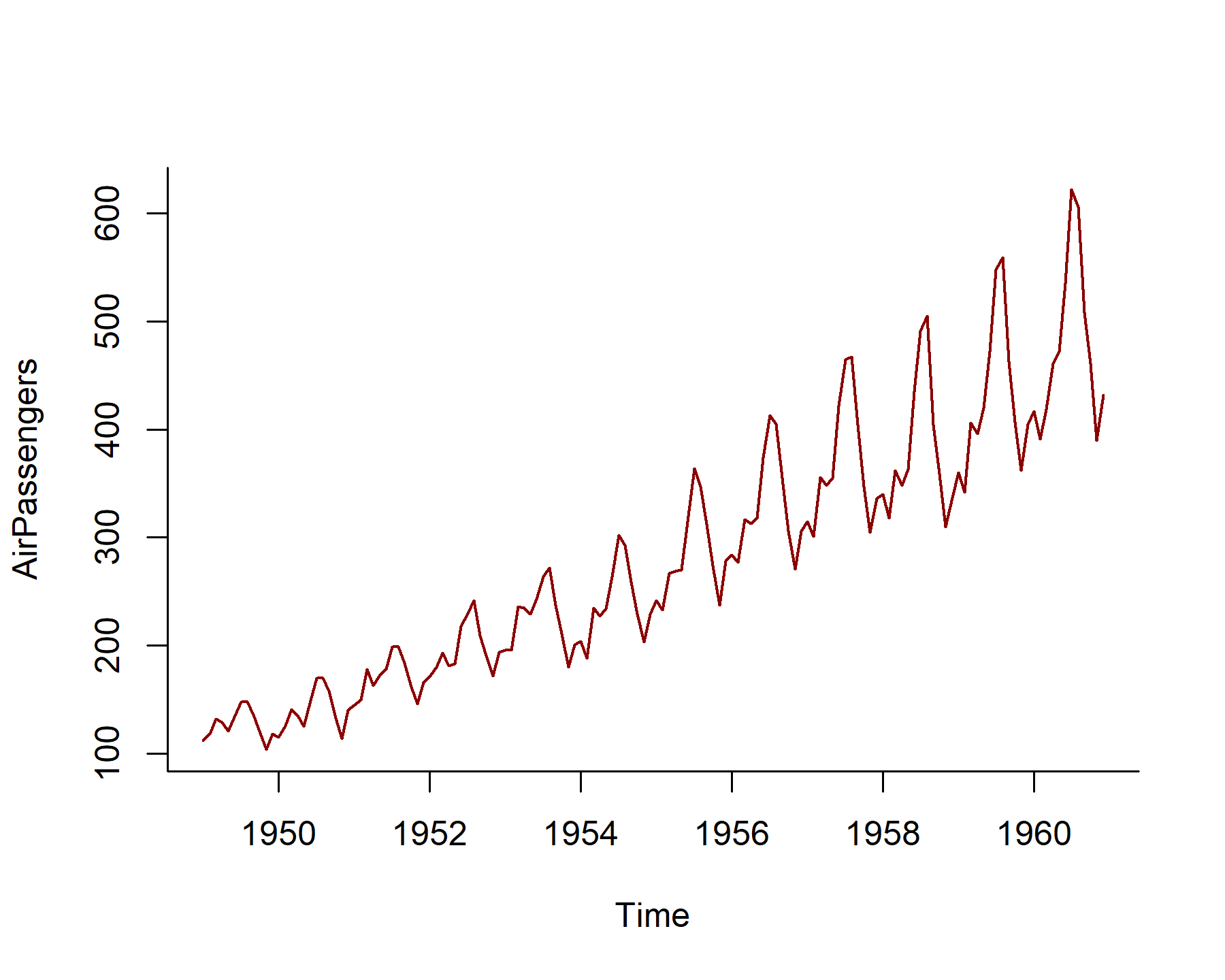
It is clear from this plot that there is strong seasonality in the passenger numers, but this pattern also appears to be changing over time. One common way to inpsect possible seasonal patterns is to calculate and plot an STL decomposition (Seasonal and Trend decomposition using Loess), which uses loess smoothing to iteratively smooth and remove certain components of the data (i.e. the long-term trend, which may be nonlinear, and the potentially time-varying seasoanality)

stl(AirPassengers, s.window = 9) %>%
  autoplot()

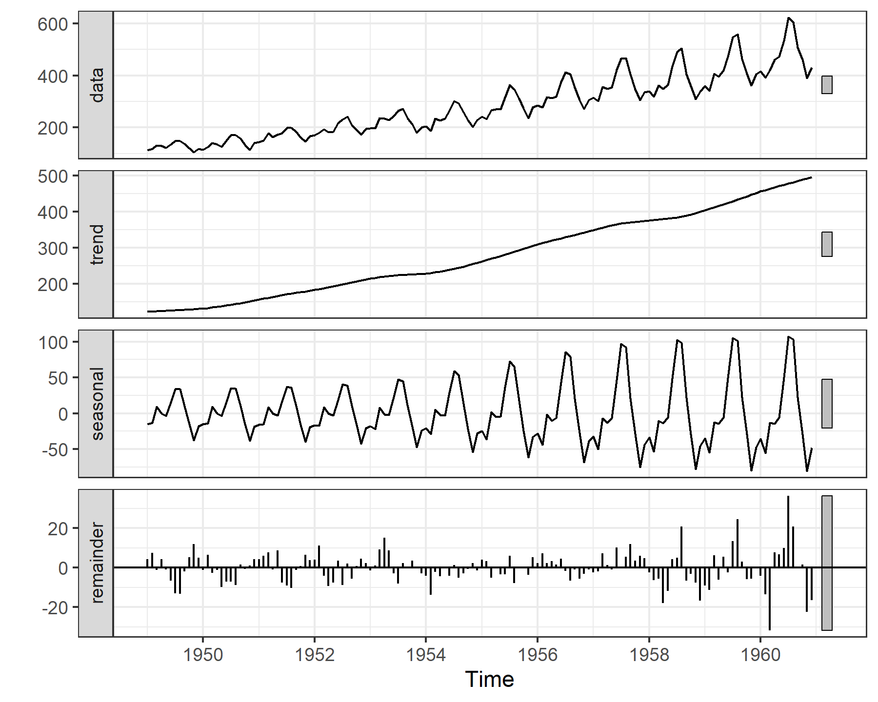
You can read about ways to modify this plot by changing the the periods over which the trend and seasonal components are smoothed using the t.window and s.window arguments, but they aren’t that important for this post. The key message is that there appears to be a long-term, nonlinear trend and a cyclic seasonal pattern that varies over time, not just in magnitude but also perhaps a bit in shape. Now for some models. First let’s convert the series to a data.frame() object that is suitable for modeling with the {mgcv} and {mvgam} packages. This function will also automatically split the data into training and testing sets, which makes it easy to evaluate different models on their forecasting abilities.

airdat <- series_to_mvgam(AirPassengers, freq = frequency(AirPassengers))
dplyr::glimpse(airdat$data_train)

## Rows: 122
## Columns: 6
## $ y      <dbl> 112, 118, 132, 129, 121, 135, 148, 148, 136, 119, 104, 118, 115…
## $ season <dbl> 1, 2, 3, 4, 5, 6, 7, 8, 9, 10, 11, 12, 1, 2, 3, 4, 5, 6, 7, 8, …
## $ year   <dbl> 1949, 1949, 1949, 1949, 1949, 1949, 1949, 1949, 1949, 1949, 194…
## $ date   <dttm> 1949-01-01 00:00:00, 1949-01-31 10:00:00, 1949-03-02 20:00:01,…
## $ series <fct> series_1, series_1, series_1, series_1, series_1, series_1, ser…
## $ time   <int> 1, 2, 3, 4, 5, 6, 7, 8, 9, 10, 11, 12, 13, 14, 15, 16, 17, 18, …

Once the data are in the correct long format, we can easily plot some features of the time series using some of {mvgam}’s S3 functions

plot_mvgam_series(data = airdat$data_train,
                  newdata = airdat$data_test)

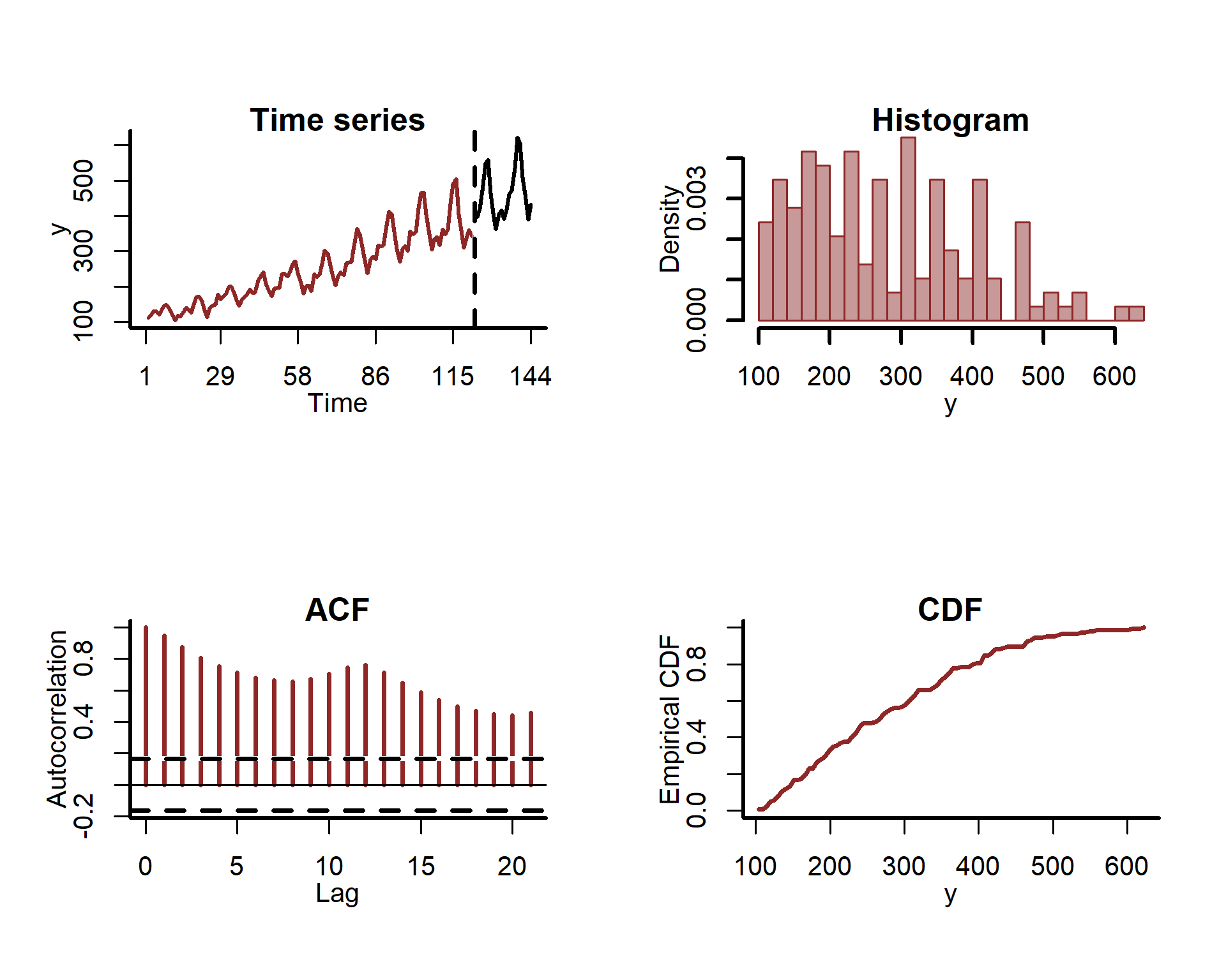
The Autocorrelation Function (ACF) plot clearly shows evidence of strong autocorrelation and seasonality, which we hope to capture in our models

Fit an mvgam model using a tensor product interaction

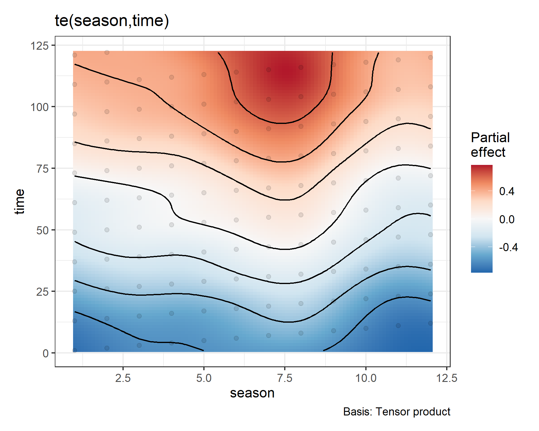
Now we can fit a model to these data to try and capture both components, i.e. the trend and seasonal patterns. Those of you familiar with {mgcv} will know that the traditional way to model time-varying effects is to use a tensor product smooth (using the te() wrapper) to capture a nonlinear interaction between ’time’ and whatever covariate we are interested in (‘season’, in this case). This is a useful first step to model smoothly-varying effects, and we have a lot of flexibility to describe the marginal effects within a te() smooth. For example, in the below model we set up the effect of ‘season’ using a cyclic smooth (bs = 'cc') that forces the seasonal pattern to begin and end in the same place (i.e. there is no discontinuity allowed at the end points of the spline, meaning that this effect constrains the smooth to be periodic).

mod1 <- mvgam(y ~ 
                # A tensor product of season and time
                te(season, time,
                   
                   # Cyclic and thin-plate marginal bases
                   bs = c('cc', 'tp'),
                   
                   # Reasonable complexities
                   k = c(8, 15)),
              
              # Define where the seasonal ends should 'join'
              knots = list(season = c(0.5, 12.5)),
              
              # Allow for overdispersion in the count series
              family = nb(),
              
              # Define the data and newdata for automatic forecasting
              data = airdat$data_train,
              newdata = airdat$data_test,
              
              # Silence printed messages
              silent = 2)

We can conveniently use gratia::draw() to view the ’time’ * ‘season’ smooth interaction function from the model’s underlying gam object (stored in the mgcv_model slot of the returned model object)

draw(mod1$mgcv_model)

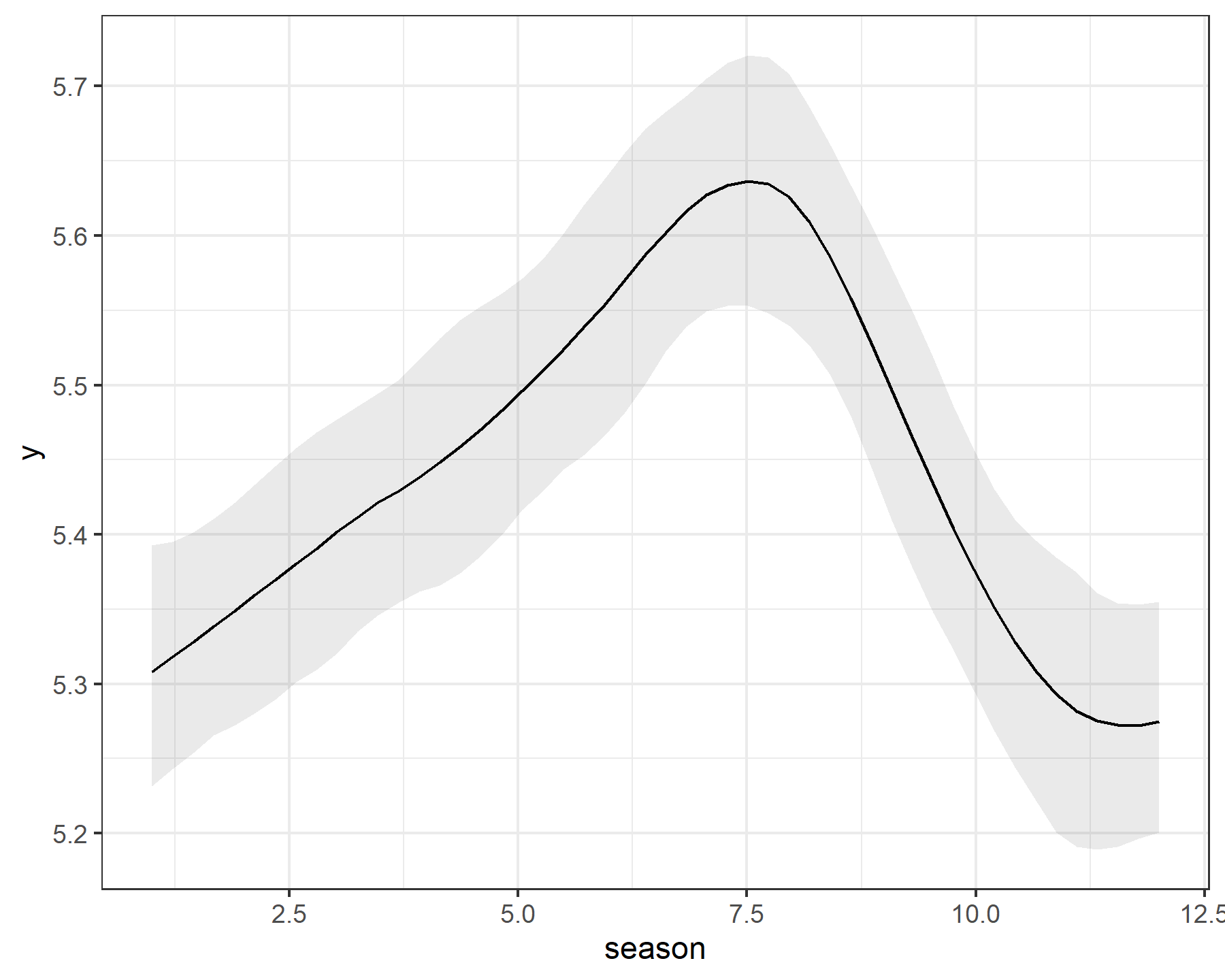
The primary seasonal pattern can be viewed using plot_predictions() from the {marginaleffects} package, which is an extremely useful package for using targeted predictions to interrogate nonlinear effects from GAMs.

plot_predictions(mod1, condition = 'season', type = 'link')

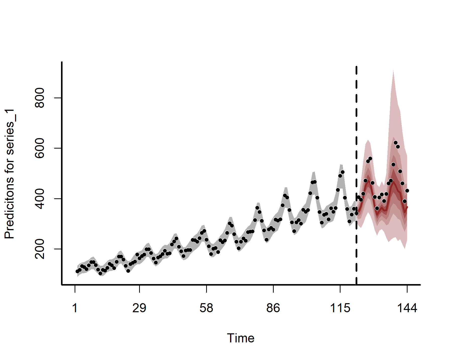
Out-of-sample forecasts from this model aren’t too bad here, but perhaps the uncertainty is a bit too wide. This is not unexpected if you take some time to understand how splines extrapolate beyond the training data

plot(mod1, type = 'forecast')

## Out of sample DRPS:
## 897.952959

This model is not too bad, but it might not be preferable for a few reasons:

1. We are capturing the temporal dimension with a spline, and we all know that splines generally give poor extrapolation behaviours
2. This model assumes that the seasonal pattern changes at the same rate that the temporal spline changes, and this might not always be the most suitable model

Using Fourier terms to capture time-varying seasonality

There is another way we can model time-varying seasonality, in this case using a Fourier transform. A Fourier series uses sets of sine and cosine terms at different frequencies, which can be weighted to approximate a huge variety of periodic functions. First compute sine and cosine functions using the forecast::fourier() function, which automatically recognises the monthly periodicity of the AirPassengers data to calculate Fourier terms of the corrrect frequencies. Here we set the order K equal to 4, which gives us a total of 8 sine and cosine predictors that we can use as regressors in our dynamic model. This sort of model is often referred to as harmonic regression because the successive Fourier terms can be thought of as representing harmonics of the previous Fourier terms.

data.frame(forecast::fourier(AirPassengers, K = 4)) %>%
  # Use clean_names as fourier() gives terrible name types
  janitor::clean_names() -> fourier_terms
dplyr::glimpse(fourier_terms)

## Rows: 144
## Columns: 8
## $ s1_12 <dbl> 0.5000000, 0.8660254, 1.0000000, 0.8660254, 0.5000000, 0.0000000…
## $ c1_12 <dbl> 0.8660254, 0.5000000, 0.0000000, -0.5000000, -0.8660254, -1.0000…
## $ s2_12 <dbl> 0.8660254, 0.8660254, 0.0000000, -0.8660254, -0.8660254, 0.00000…
## $ c2_12 <dbl> 0.5, -0.5, -1.0, -0.5, 0.5, 1.0, 0.5, -0.5, -1.0, -0.5, 0.5, 1.0…
## $ s3_12 <dbl> 1, 0, -1, 0, 1, 0, -1, 0, 1, 0, -1, 0, 1, 0, -1, 0, 1, 0, -1, 0,…
## $ c3_12 <dbl> 0, -1, 0, 1, 0, -1, 0, 1, 0, -1, 0, 1, 0, -1, 0, 1, 0, -1, 0, 1,…
## $ s4_12 <dbl> 0.8660254, -0.8660254, 0.0000000, 0.8660254, -0.8660254, 0.00000…
## $ c4_12 <dbl> -0.5, -0.5, 1.0, -0.5, -0.5, 1.0, -0.5, -0.5, 1.0, -0.5, -0.5, 1…

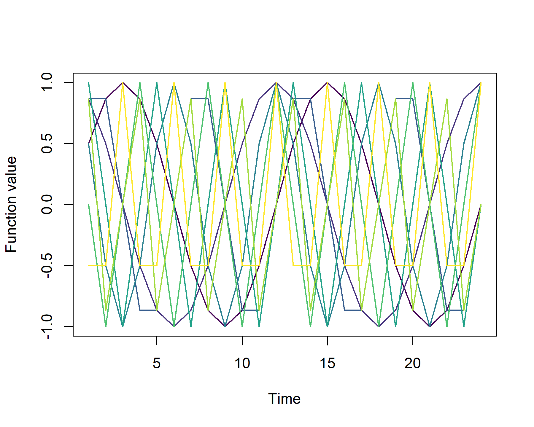
Viewing these Fourier terms (for the first 24 time points) gives a sense of how they can be thought of as a particular type of basis expansion

matplot(as.matrix(fourier_terms)[1:24,], type = 'l',
        ylab = 'Function value', xlab = 'Time',
        col = viridis::viridis(8), lty = 1, lwd = 1.5)

airdat$data_train = airdat$data_train %>%
  dplyr::bind_cols(fourier_terms[1:NROW(airdat$data_train), ])
airdat$data_test = airdat$data_test %>%
  dplyr::bind_cols(fourier_terms[(NROW(airdat$data_train) + 1):
                                   NROW(fourier_terms), ])

Next we can fit an mvgam() model that includes a smooth nonlinear temporal trend and time-varying seasonality, but using the Fourier terms in place of the cyclic smooth like we did above. This is done by first using a monotonic smooth of ’time’ that ensures the temporal trend never declines, which seems appropriate here. The {mvgam} package includes options for monotonically increasing or monotonically decreasing smooths using the moi and mod basis constructors. This is a nice feature that is difficult to incorporate in normal GAMs fitted in either {mgcv} or {brms}. The time-varying seasonality is captured by allowing the coefficients on the Fourier terms to vary over time using separate splines that take advantage of the 'by' argument in the s() wrapper. This effectively sets up independent smooths of ’time’ that are then interacted with the Fourier terms, formulating a time-varying coefficient model for each Fourier term.

mod2 <- mvgam(y ~ 
                # Monotonic smooth of time to ensure the trend
                # either increases or flattens, but does not 
                # decrease
                s(time, bs = 'moi', k = 10) +
                
                # Time-varying fourier coefficients to capture
                # possibly changing seasonality
                s(time, by = s1_12, k = 5) +
                s(time, by = c1_12, k = 5) +
                s(time, by = s2_12, k = 5) +
                s(time, by = c2_12, k = 5) +
                s(time, by = s3_12, k = 5) +
                s(time, by = c3_12, k = 5),
              
              # Response family and data as before
              family = nb(),
              data = airdat$data_train,
              newdata = airdat$data_test,
              silent = 2)

Of course this model still uses a spline of ’time’ for the trend, but the monotonic restriction ensures that the predictions are at least somewhat controllable. This second model is preferred based on in-sample fits, which we can readily compare using the Approximate Leave-One-Out Cross-Validation with functionality from the wonderful {loo} package. A higher Expected Log Predictive Density (ELPD) is preferred here

loo_compare(mod1, mod2)

##      elpd_diff se_diff
## mod2   0.0       0.0  
## mod1 -16.8       2.8

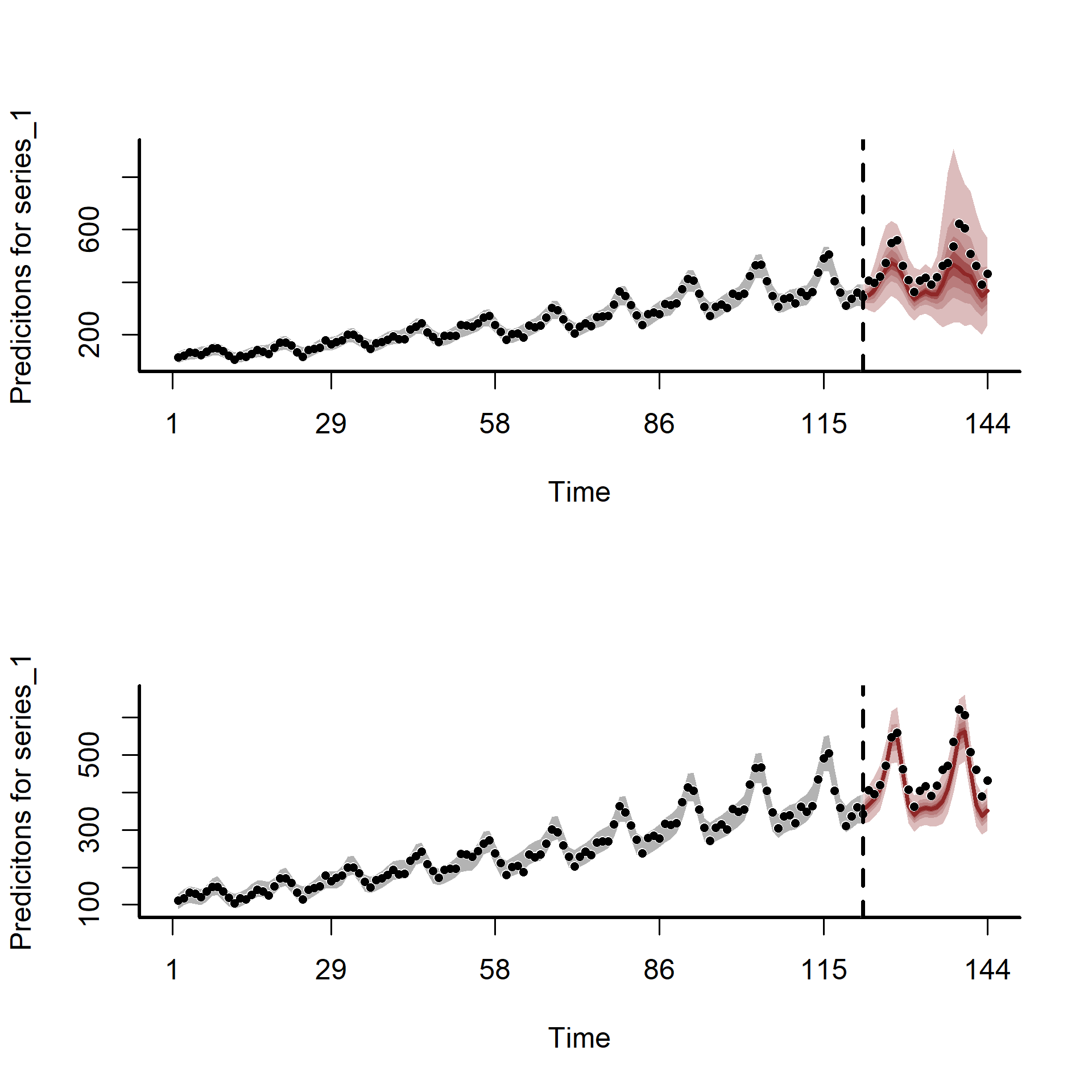
But what about forecasts? Here we plot out-of-sample forecasts from both models, which again show that the second model is slightly preferred

layout(matrix(1:2, nrow = 2))
plot(mod1, type = 'forecast')

## Out of sample DRPS:
## 897.952959

plot(mod2, type = 'forecast')

## Out of sample DRPS:
## 667.239806

layout(1)

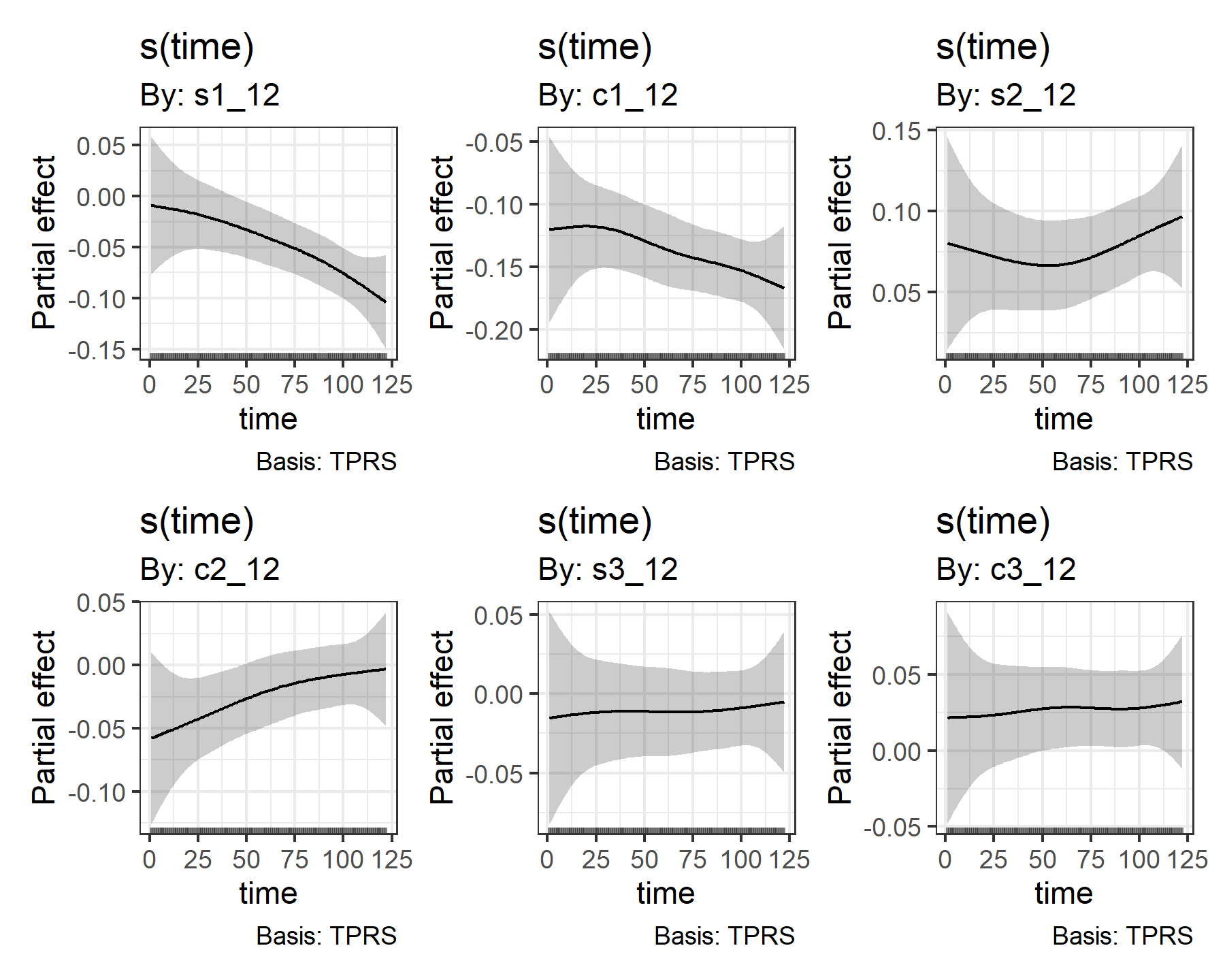
Look at the partial effect plots for the smooths to see how some of the Fourier coefficients are estimated to change over time

gratia::draw(mod2$mgcv_model, select = 2:7)

Plotting trend and seasonal components from a harmonic regression

Plotting this model takes a bit more work, as we need to use targeted predictions from the model to visualise the two primary effects (i.e. the nonlinear trend and the time-varying seasonality).

First a plot of the trend, which can be done easily in this model using the 'condition' argument in plot_predictions() to compute expectations from the model (i.e. predictions on the outcome scale, but ignoring the overdispersion parameter from the Negative Binomial sampling distribution)

p1 <- plot_predictions(mod2, 
                       condition = 'time', 
                       type = 'expected') +
  labs(y = 'Expected passengers',
       x = '',
       title = 'Long-term trend')

And now the time-varying seasonal pattern, which requires subtracting the conditional trend predictions from the total predictions

with_season <- predict(mod2, summary = FALSE,
                       type = 'expected')
agg_over_season <- predict(mod2, 
                           newdata = datagrid(model = mod2,
                                              time = unique),
                           summary = FALSE,
                           type = 'expected')
season_preds <- with_season - agg_over_season
p2 <- ggplot(airdat$data_train %>%
               dplyr::mutate(pred = apply(season_preds, 2, mean),
                             upper = apply(season_preds, 2, function(x) 
                               quantile(x, probs = 0.975)),
                             lower = apply(season_preds, 2, function(x) 
                               quantile(x, probs = 0.025))),
             aes(x = time, y = pred)) +
  geom_ribbon(aes(ymax = upper,
                  ymin = lower),
              alpha = 0.2) +
  geom_line()+
  labs(y = 'Expected passengers',
       title = 'Time-varying seasonality')

We can now plot these effects together using functionality from the {patchwork} package

p1 + p2 + plot_layout(ncol = 1)

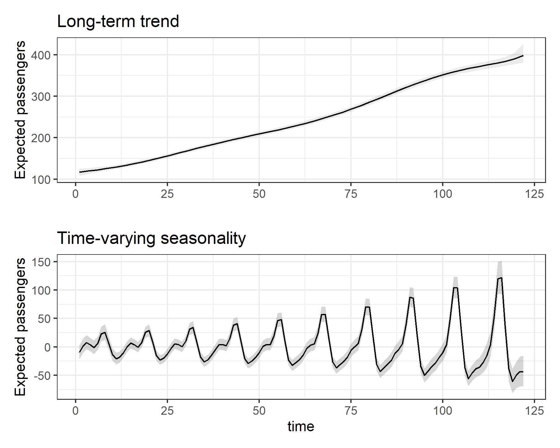
This plot clearly shows how the model has estimated both components, and that the seasonal pattern changes in both shape and magnitude over time

Time-varying periodicity?

The above example shows how Fourier terms can be used to capture time-varying seasonality. But what if the periodicity itself is changing over time? In other words, how might we model a series that starts out with regular periodic variation that occurs every ~ 8 weeks but that proceeds to show a shrinking or expanding periodic window? Below is a very brief example of how we could expand the Fourier strategy to potentially model this

First, I define function to construct monotonically increasing or decreasing coefficients. This will be helpful to simulate time-varying periodicity

monotonic_fun = function(times, k = 4){
  x <- sort(as.vector(scale(times)))
  exp(k * x) / (1 + exp(k * x))
}

Now for the simulation, which involves constructing Fourier series for two different periodicities (k = 12 and k = 6 in this example), each with three Fourier terms. I then simulate time-varying coefficients for these terms, forcing the period-12 terms to decline toward zero over time while allowing the period-6 terms to increase over time. These coefficients, together with the simulated Fourier terms themselves, should give us the ingredients to simulate a time series in which the periodicity shrinks from ~12 to ~6 over time

set.seed(123)
times <- 1:120

# Construct Fourier series for two different periodicities
data.frame(forecast::fourier(ts(times, frequency = 12), K = 3)) %>%
  dplyr::bind_cols(forecast::fourier(ts(times, frequency = 6), K = 3)) %>%
  # Use clean_names as fourier() gives terrible name types
  janitor::clean_names() -> fourier_terms

# Create the time-varying Fourier coefficients
betas <- matrix(NA, nrow = length(times), ncol = NCOL(fourier_terms))

# Period 12 coefficients drop montonically toward zero over time
p12_names <- grep('_12', names(fourier_terms), fixed = TRUE)
for(i in p12_names){
  betas[, i] <- monotonic_fun(times, k = runif(1, -3, -0.25))
}

# Period 6 coefficients increase monotonically over time
p6_names <- grep('_6', names(fourier_terms), fixed = TRUE)
for(i in p6_names){
  betas[, i] <- monotonic_fun(times, k = runif(1, 0.25, 3))
}

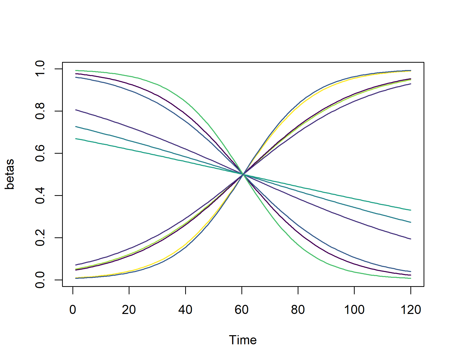
Plot the Fourier coefficients through time

matplot(betas, type = 'l', xlab = 'Time',
        col = viridis::viridis(8), lty = 1, lwd = 1.5)

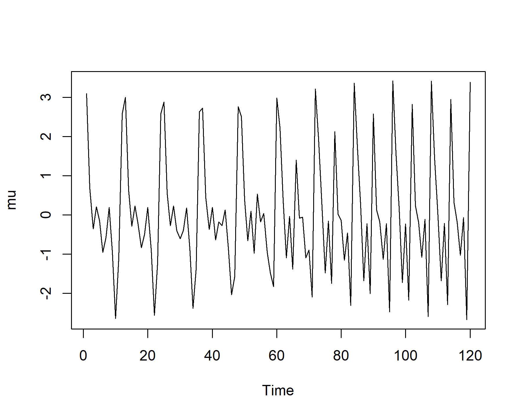
Now calculate the linear predictor and plot it

mu <- vector(length = length(times))
for(i in 1:length(times)){
  mu[i] <- as.matrix(fourier_terms)[i, ] %*% betas[i, ] 
}
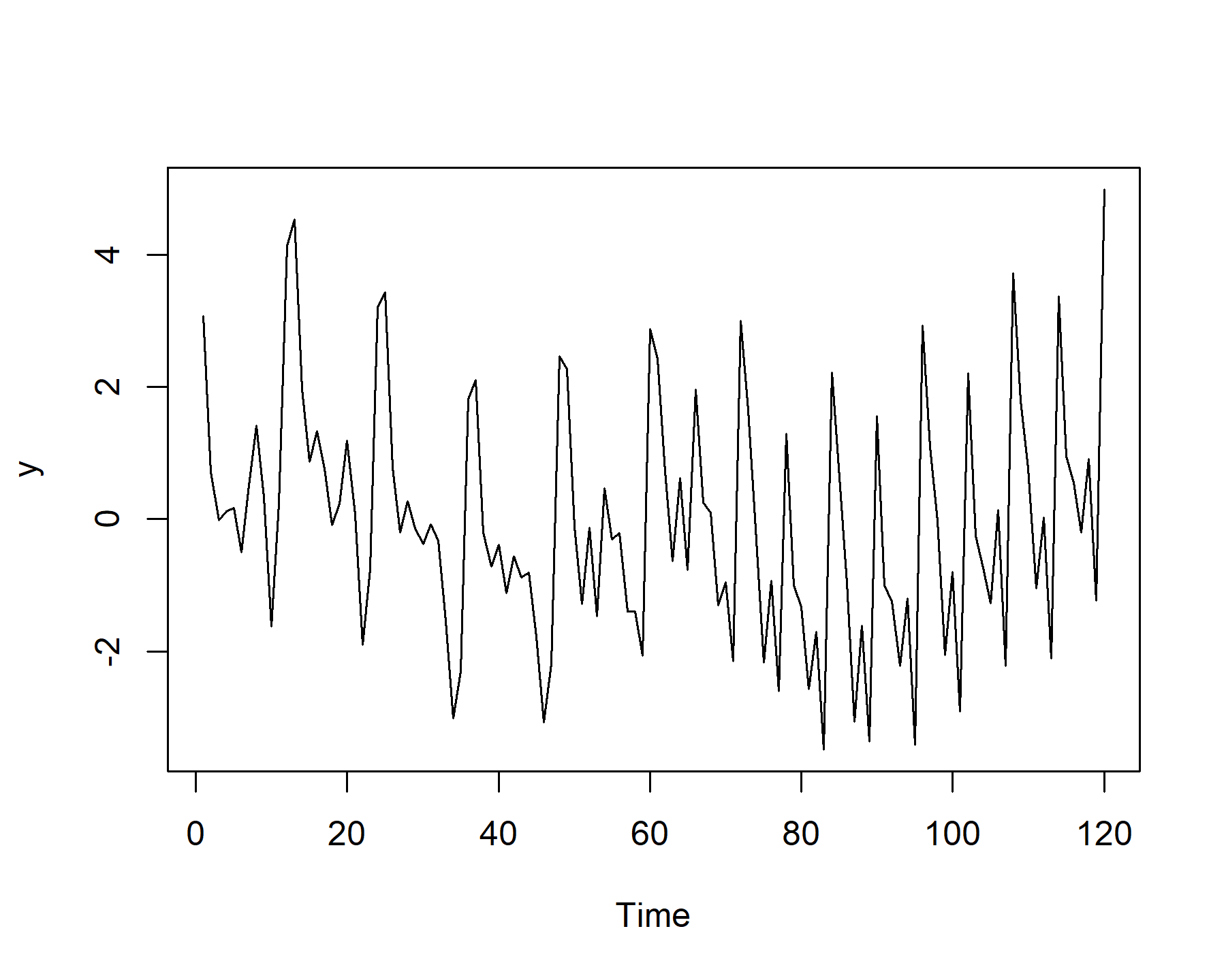
plot(mu, type = 'l', xlab = 'Time')

Finally, add some Gaussian Random Walk noise and plot the resulting simulated time series

y <- mu + cumsum(rnorm(length(times), sd = 0.25))
plot(y, type = 'l', xlab = 'Time')

Now we can construct the data for modeling; this assumes we’ve thought carefully about the problem and have included the Fourier series for both periodicities as predictors

dat <- data.frame(y, time = times) %>%
  dplyr::bind_cols(fourier_terms)

And we can now fit the dynamic GAM, which uses a State-Space representation to capture time-varying seasonality, periodicity and the Random Walk autocorrelation process

mod3 <- mvgam(
  
  # Observation formula; empty
  formula = y ~ -1,
  
  # Process formula contains the seasonal terms
  trend_formula = ~
    
    # Time-varying fourier coefficients to capture
    # possibly changing seasonality AND periodicity
    s(time, by = s1_12, k = 5) +
    s(time, by = c1_12, k = 5) +
    s(time, by = s2_12, k = 5) +
    s(time, by = c2_12, k = 5) +
    s(time, by = s3_12, k = 5) +
    s(time, by = c3_12, k = 5) +
    s(time, by = s1_6, k = 5) +
    s(time, by = c1_6, k = 5) +
    s(time, by = s2_6, k = 5) +
    s(time, by = c2_6, k = 5) +
    s(time, by = c3_6, k = 5),
  
  # Random walk for the trend
  trend_model = RW(),
  
  # Gaussian observations
  family = gaussian(),
  
  # Realistic priors on variance components
  priors = c(prior(exponential(2),
                   class = sigma),
             prior(exponential(2),
                   class = sigma_obs)),
  
  # Sampler settings
  burnin = 1000,
  samples = 1000,
  silent = 2,
  
  # Data
  data = dat)

Plot the time-varying Fourier coefficients as before, using gratia::draw()

gratia::draw(mod3$trend_mgcv_model)

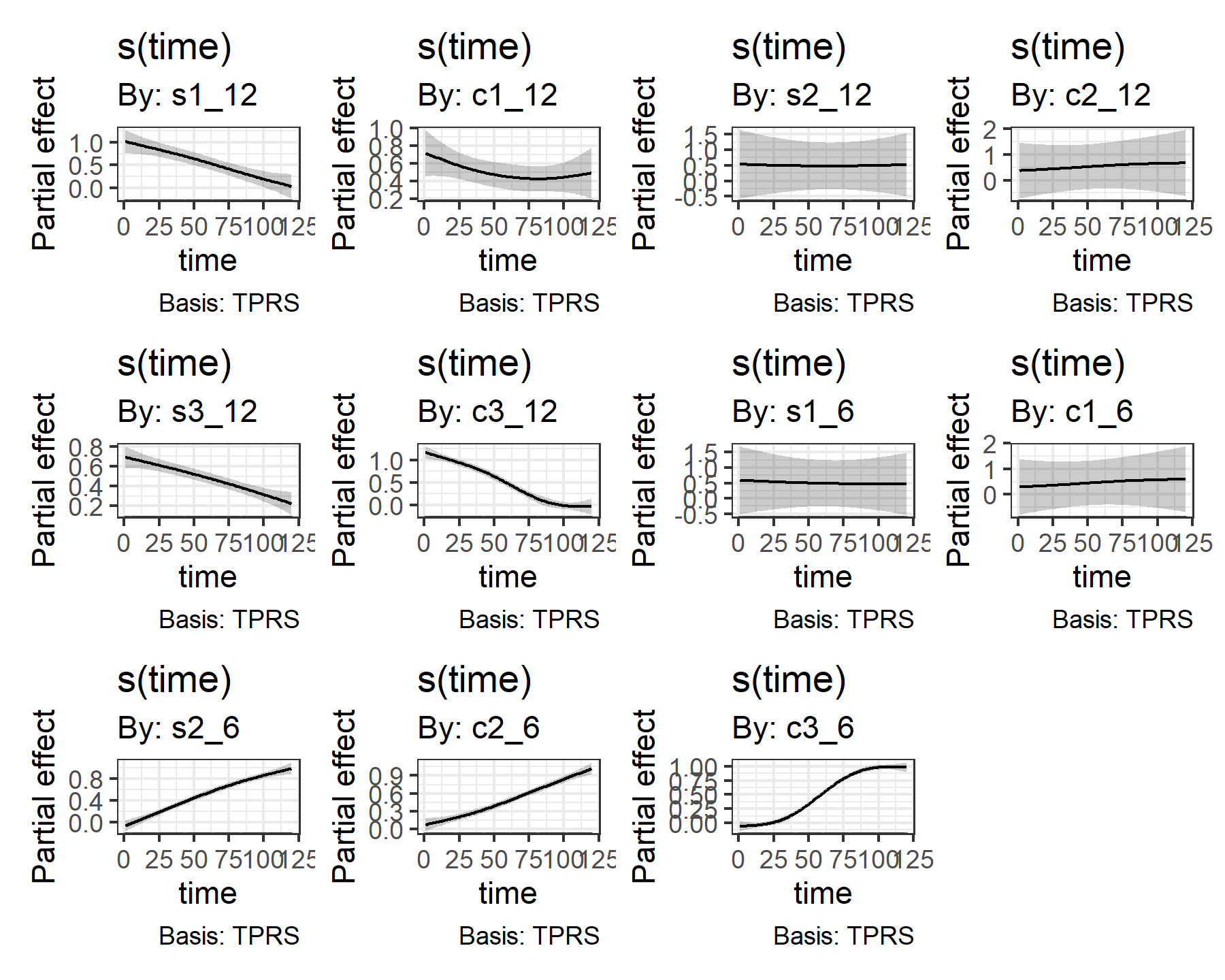
As before, our model has successfully captured the time-varying coefficients for these terms. Notice how many of the period-12 terms (i.e. s1_12 and c3_12) are estimated to decline over time, while many of the period-6 terms (i.e. s2_6 and c3_6) are estimated to increase over time. It is encouraging that the model has been able to find these while also dealing with the Random Walk autocorrelation process and the two variance terms (process error and observation error).

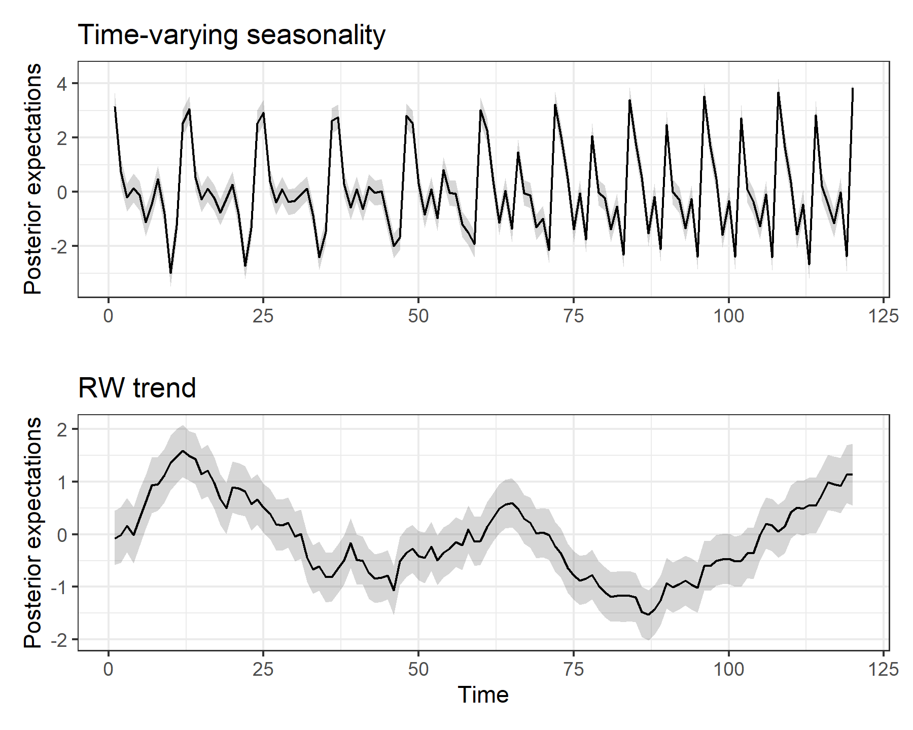
We can also plot the time-varying seasonality using posterior expectations as we did for the first example above. But note that this plot does not include the Random Walk component in its predictions

season_preds <- predict(mod3, summary = FALSE,
                        type = 'expected')
p1 <- ggplot(dat %>%
         dplyr::mutate(pred = apply(season_preds, 2, mean),
                       upper = apply(season_preds, 2, function(x) 
                         quantile(x, probs = 0.975)),
                       lower = apply(season_preds, 2, function(x) 
                         quantile(x, probs = 0.025))),
       aes(x = time, y = pred)) +
  geom_ribbon(aes(ymax = upper,
                  ymin = lower),
              alpha = 0.2) +
  geom_line() +
  labs(y = 'Posterior expectations',
       x = '',
       title = 'Time-varying seasonality')

Now we can extract the RW trend that was estimated and subtract the seasonal predictions, which will give us a view of the potentially nonlinear trend that was estimated by the model

trend_preds <- hindcast(mod3, type = 'expected')$hindcasts[[1]] - 
  season_preds

p2 <- ggplot(dat %>%
         dplyr::mutate(pred = apply(trend_preds, 2, mean),
                       upper = apply(trend_preds, 2, function(x) 
                         quantile(x, probs = 0.975)),
                       lower = apply(trend_preds, 2, function(x) 
                         quantile(x, probs = 0.025))),
       aes(x = time, y = pred)) +
  geom_ribbon(aes(ymax = upper,
                  ymin = lower),
              alpha = 0.2) +
  geom_line() +
  labs(y = 'Posterior expectations',
       x = 'Time',
       title = 'RW trend')

Once again, we can plot the two together using {patchwork}

p1 + p2 + plot_layout(ncol = 1)

This post has hopefully given you some ideas about useful modeling strategies for dealing with time-varying seasonality. Of course, we may want to try and explain why seasonality varies over time. In that case, I often find distributed lag predictors to be especially helpful. Thanks for reading!

Further reading

The following papers and resources offer useful material about Dynamic Harmonic Regression and using GAMs for time series modeling / forecasting

Autin, M. A., & Edwards, D. Nonparametric harmonic regression for estuarine water quality data Environmetrics 21.6 (2010): 588-605.

Karunarathna, K. A. N. K., Wells, K., & Clark, N. J. (2024). Modelling nonlinear responses of a desert rodent species to environmental change with hierarchical dynamic generalized additive models. Ecological Modelling, 490, 110648.

Young, P. C., Pedregal, D. J., & Tych, W. (1999). Dynamic harmonic regression. Journal of Forecasting, 18, 369–394.