Using Stan to model geostatistical count data with distance matrices
By Nicholas Clark in stan simulation
November 16, 2023
Required libraries
cmdstanr
MASS
raster
ggplot2
viridis
Purpose and model introduction
This script simulates Poisson observations of an underlying spatially autocorrelated data generating process. It also provides Stan code for estimating parameters of the model in a Bayesian framework. Observations \(\boldsymbol{Y}\) are assumed to be drawn from a Poisson distribution with location \(\lambda\):
$$for\:i=1,...,N$$
$$\boldsymbol{Y}_{i}\sim \text{Poisson}(\lambda_{i})$$
A linear predictor is modeled on the \(log\) scale to capture effects of covariates and a spatial effect on \(\lambda\):
$$log(\lambda)={\beta}*\boldsymbol{X}+\phi$$
\(\beta\) is the set of regression coefficients that describe associations between predictor variables in the model design matrix \(\boldsymbol{X}\) and \(log(\lambda)\). \(\phi\) captures spatial effects, which can be modeled using a wide variety of functions (i.e. splines, hierarchical intercepts indexed by region, Gaussian Processes etc…). In this example, we use a spatial Gaussian Process with squared exponential covariance kernel:
$$\phi\sim \text{MultiNormal}(0, \Sigma)$$
\(\Sigma\) is a covariance matrix with:
$$\Sigma[i, j] = \alpha^ 2* exp(-0.5 * ((\boldsymbol{distances[i, j]} / \rho))^2),~if~~i~!= j$$
$$\Sigma[i, j] = \alpha^ 2,~if~~i~= j$$
The term \(exp(-0.5 * ((\boldsymbol{distances[i, j]} / \rho)) ^ 2)\) is the spatial kernel function and depends on \(\rho\) (often called the length scale parameter), which controls how quickly the correlations between spatial points decay as a function of geographical distance (in km). The parameter \(\alpha\) controls the marginal variability of the spatial function at all points; in other words it controls how much the spatial term contributes to the linear predictor.
Define the joint probabilistic model
First we will define the Stan model code for estimating parameters under the model outlined above.
gp_stan_code <-
'
functions {
  // Function to compute the squared exponential covariance matrix and
  // take the cholesky decomposition for more efficient computation
  // of multivariate normal realisations
  matrix L_cov_exp_quad_dis(
          int N,
          matrix distances,
			    real alpha,
			    real rho,
			    real delta) {
    matrix[N, N] Sigma;
    Sigma = square(alpha) * exp(-0.5 * (square(distances / rho))) +
            diag_matrix(rep_vector(delta, N));
    return cholesky_decompose(Sigma);
  }
}

data {
    int N;                    // total number of observations
    matrix[N, N] distances;   // distance matrix (in km)
    int K;                    // number of columns in the model matrix
    matrix[N,K] X;            // the model matrix
    array[N] int<lower=0> y;  // the response variable (as non-negative integers)
}

transformed data {
  // Small offset to ensure the covariance matrix is positive definite
  real delta = 1e-9;
}

parameters {
  // Define any unknown parameters to be sampled
  vector[K] beta;
  real<lower=0> rho;
  real<lower=0> alpha;
  vector[N] eta;
}

transformed parameters {
  // Calculate the latent Gaussian process function (phi)
  matrix[N, N] L_chol = L_cov_exp_quad_dis(N, distances, alpha, rho, delta);
  vector[N] gp_function = L_chol * eta;
}

model {
  // Prior for the GP length scale (i.e. spatial decay)
  // very small values will be inidentifiable, so an informative prior
  // is a must
  rho ~ normal(2, 2.5);
  // Prior for the GP covariance magnitude
  alpha ~ std_normal();
  // Multiplier for non-centred GP parameterisation
  eta ~ std_normal();

  // Likelihood, where the linear
  // predictor is an additive combination of the latent GP and
  // fixed effects of covariates
  y ~ poisson_log(X * beta + gp_function);
}
'
Load cmdstanr and compile the model to C++ code. See
information here for troubleshooting advice when installing Stan and Cmdstan
library(cmdstanr)
cmd_mod <- cmdstan_model(write_stan_file(gp_stan_code),
                         stanc_options = list('canonicalize=deprecations,braces,parentheses'))
Simulate spatially autocorrelated Poisson data
Now that the model is defined in Stan language, we need to simulate data to explore the model. We simulate 150 geospatial coordinates in roughly the Brisbane, Queensland area
N <- 150
lat <- runif(n = N, min = -27.65, max = -27)
lon <- runif(n = N, min = 152.8, 153)
coords <- as.matrix(cbind(lon, lat))
colnames(coords) <- c('Longitude', 'Latitude')
Now simulate a precipitation variable and assign a positive coefficient for its effect on the process. We use a standard normal distribution for this simulation: \(\boldsymbol{precip}\sim \text{Normal}(0,1)\). This is useful as it mimics what we might see if we took a continuous variable and standardised it to unit variance. Many texts suggest you should do this for computational reasons. But really it just helps a bit for specifying priors
precip <- rnorm(N)
beta_precip <- 0.3
Assign Gaussian Process parameter values to ensure there is obvious spatial autocorrelation (with spatial decay \(\rho = 5km\))
alpha <- 1
rho <- 5
Calculate distances (in meters) between the points and ensure the resulting matrix is symmetric
library(raster)
m <- pointDistance(coords, lonlat = TRUE)
m[upper.tri(m)] = t(m)[upper.tri(m)]
## Warning: package 'raster' was built under R version 4.3.2
## Loading required package: sp
## Warning: package 'sp' was built under R version 4.3.2
Convert distance (which is in meters) to kilometers and preview the distance matrix
m <- m / 1000
m[1:6, 1:6]
##           [,1]      [,2]      [,3]      [,4]      [,5]      [,6]
## [1,]  0.000000 25.444495  7.862131 16.876604 10.948461 17.707530
## [2,] 25.444495  0.000000 19.031165 19.933376 15.710278  8.403163
## [3,]  7.862131 19.031165  0.000000  9.997982  3.407973 12.572540
## [4,] 16.876604 19.933376  9.997982  0.000000  9.301197 17.395006
## [5,] 10.948461 15.710278  3.407973  9.301197  0.000000  9.840844
## [6,] 17.707530  8.403163 12.572540 17.395006  9.840844  0.000000
range(m)
## [1] 0.00000 69.91692
Calculate the Gaussian Process squared exponential covariance matrix. A small offset is used on the diagonals to ensure the resulting matrix is Positive-Definite. This is a requirement for simulating multivariate normal draws. Preview the covariance matrix
K <- alpha ^ 2 * exp(-0.5 * ((m / rho) ^ 2)) + diag(1e-9, N)
K[1:6, 1:6]
##              [,1]         [,2]         [,3]         [,4]        [,5]
## [1,] 1.000000e+00 2.379914e-06 0.2904679164 0.0033580483 0.090956308
## [2,] 2.379914e-06 1.000000e+00 0.0007146594 0.0003537961 0.007181431
## [3,] 2.904679e-01 7.146594e-04 1.0000000010 0.1354445399 0.792719718
## [4,] 3.358048e-03 3.537961e-04 0.1354445399 1.0000000010 0.177240942
## [5,] 9.095631e-02 7.181431e-03 0.7927197180 0.1772409416 1.000000001
## [6,] 1.890087e-03 2.435914e-01 0.0423674335 0.0023537992 0.144158155
##             [,6]
## [1,] 0.001890087
## [2,] 0.243591437
## [3,] 0.042367433
## [4,] 0.002353799
## [5,] 0.144158155
## [6,] 1.000000001
Simulate the latent Gaussian Process function as random draws from a zero-centred multivariate normal distribution with K as the covariance matrix
sim_gp <- MASS::mvrnorm(1, mu = rep(0, N), Sigma = K)
Now we can finally simulate the observed counts, which follow the linear predictor we set out at the beginning of this tutorial
sim_y <- rpois(N, lambda = exp(sim_gp + beta_precip * precip))
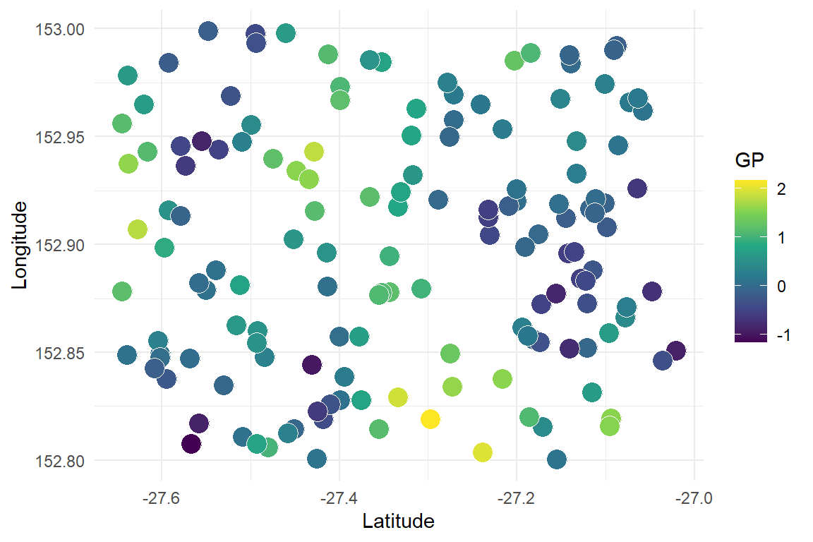
Plot the data to observe the spatial pattern. First plot the latent function, which should show obvious spatial autocorrelation
library(ggplot2)
## Warning: package 'ggplot2' was built under R version 4.3.3
ggplot(data.frame(Y = sim_y,
                  GP = sim_gp,
                  Longitude = lon,
                  Latitude = lat),
       aes(x = Latitude, y = Longitude, fill = GP)) +
  geom_point(size = 5, shape = 21, col = 'white') +
  scale_fill_continuous(type = "viridis") +
  theme_minimal()
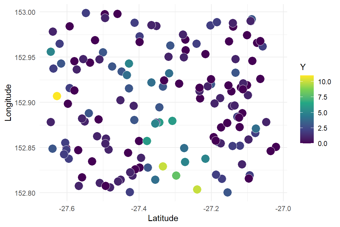
Now plot the integer observations, which are naturally messier
ggplot(data.frame(Y = sim_y,
                  GP = sim_gp,
                  Longitude = lon,
                  Latitude = lat),
       aes(x = Latitude, y = Longitude, fill = Y)) +
  geom_point(size = 5, shape = 21, col = 'white') +
  scale_fill_continuous(type = "viridis") +
  theme_minimal()
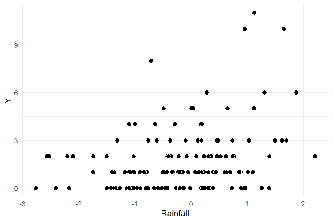
It is also worth plotting the observations against the predictors (precipitation, in this case)
ggplot(data.frame(Y = sim_y,
                  Rainfall = precip),
       aes(x = Rainfall, y = Y)) +
  geom_point(size = 2.5, shape = 21, col = 'white', fill = 'black') +
  theme_minimal()
Fit a standard Generalized Linear Model to simulated data
We can quickly understand why it is problematic to ignore spatial variation (or any kind of systematic heterogeneity) when fitting models. Start with a basic Poisson GLM that ignores the spatial component. Generally I would not advocate mixing Maximum Likelihood and Bayesian models. In my view, Bayesian is better because it forces us to think more deeply about the model and its connections to both data and prior knowledge. But a quick glm, which uses iteratively reweighted least squares to find the Maximum Likelihood estimates of a Generalized Linear Model, will be fine for our purposes here
nonspat_mod <- glm(sim_y ~ precip, family = poisson())
summary(nonspat_mod)
##
## Call:
## glm(formula = sim_y ~ precip, family = poisson())
##
## Coefficients:
##             Estimate Std. Error z value Pr(>|z|)
## (Intercept)  0.50320    0.06460   7.789 6.74e-15 ***
## precip       0.39753    0.06919   5.745 9.18e-09 ***
## ---
## Signif. codes:  0 '***' 0.001 '**' 0.01 '*' 0.05 '.' 0.1 ' ' 1
##
## (Dispersion parameter for poisson family taken to be 1)
##
##     Null deviance: 321.86  on 149  degrees of freedom
## Residual deviance: 287.95  on 148  degrees of freedom
## AIC: 554.01
##
## Number of Fisher Scoring iterations: 5
Visualise the estimated precipitation regression coefficient \(\beta_{precip}\). First, define some colours for nice plots
c_light <- c("#DCBCBC")
c_light_highlight <- c("#C79999")
c_mid <- c("#B97C7C")
c_mid_highlight <- c("#A25050")
c_dark <- c("#8F2727")
c_dark_highlight <- c("#7C0000")
Because we fit the model using a form of maximum likelihood, parameter uncertainty can be recovered using the model’s assumed multivariate normal posterior distribution
coef_posteriors <- MASS::mvrnorm(2000,
                                 mu = coef(nonspat_mod),
                                 Sigma = vcov(nonspat_mod))
Plot the estimates for \(\beta_{precip}\) and overlay the true simulated value in black
hist(coef_posteriors[,2],
     col = c_mid_highlight, border = 'white', lwd = 2,
     main = '', yaxt = 'n', ylab = '', xlab = expression(beta[precip]))
abline(v = beta_precip, lwd = 3.5, col = 'white')
abline(v = beta_precip, lwd = 3, col = 'black')
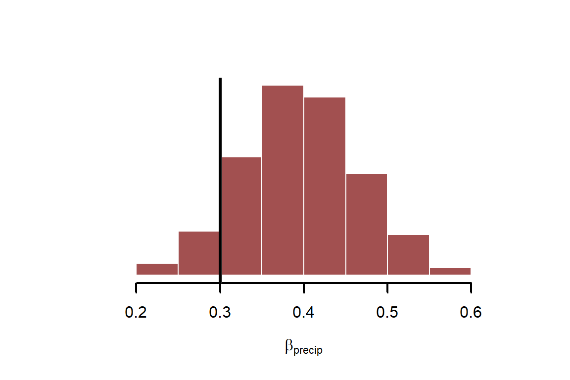
This parameter seems to be recovered well. But how do model residuals look?
qqnorm(residuals(nonspat_mod), pch = 16, ylim = c(-6, 6),
       bty = 'l', col = c_mid_highlight)
qqline(residuals(nonspat_mod), lwd = 2)
box(bty = 'l', lwd = 2)
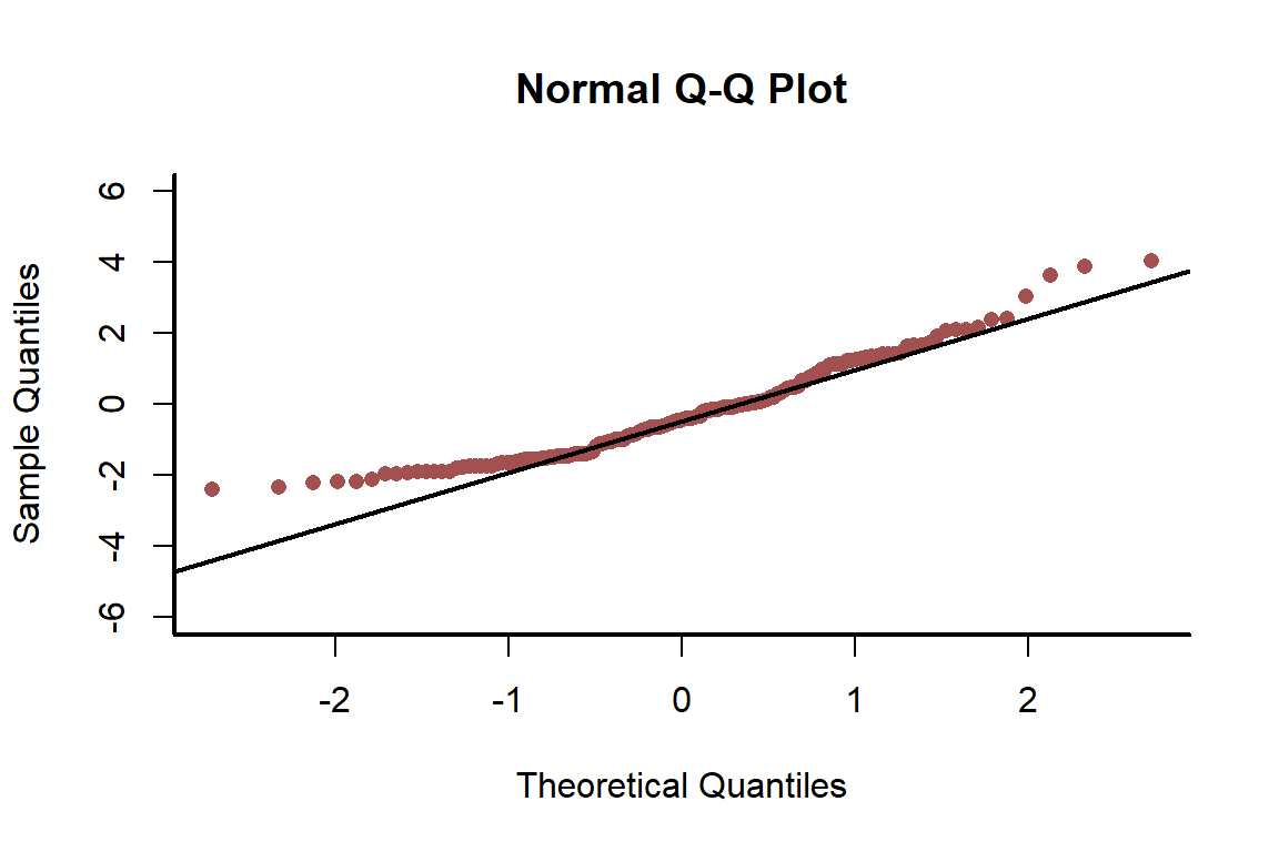
The model is not capturing the dispersion in the data. This suggests there is a problem. Plot residuals against observed values to see if there are any obvious patterns
plot(sim_y, residuals(nonspat_mod),pch = 16,
     bty = 'l', col = c_mid_highlight,
     ylab = 'Residuals',
     xlab = 'Observed counts')
box(bty = 'l', lwd = 2)
abline(h = 0, lwd = 3, col = 'white')
abline(h = 0, lwd = 2.5)
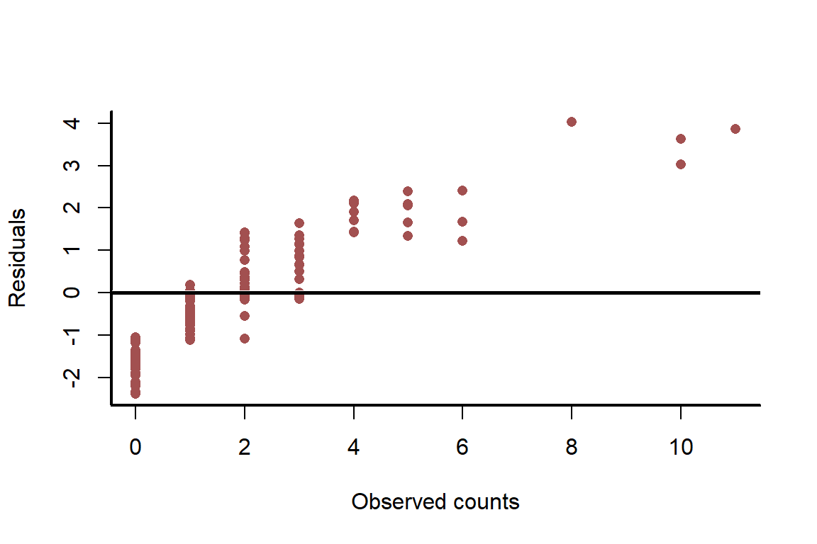
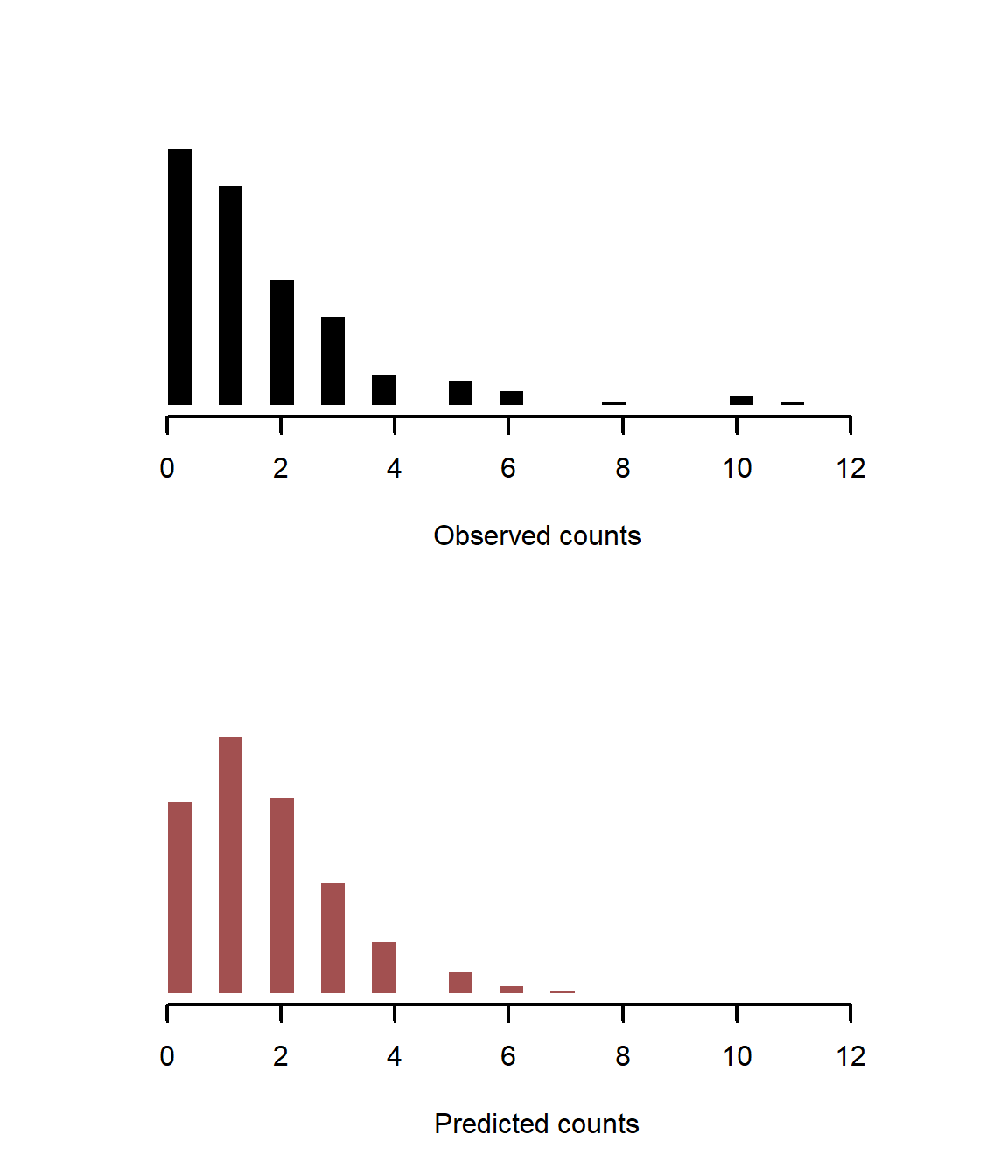
Another useful plot is to compare simulated counts to observed counts, which more closely inspects whether our simulations capture properties of the observed data
preds <- matrix(NA, nrow = 2000, ncol = length(sim_y))
for(i in 1:2000){
  preds[i, ] <- rpois(length(sim_y),
                      lambda = exp(coef_posteriors[i, 1] +
                                     coef_posteriors[i, 2] * precip))
}
layout(matrix(1:2))
hist(sim_y, col = 'black',
     freq = F,
     breaks = seq(0, pmax(max(sim_y), max(preds)), length.out = 30),
     border = 'white', lwd = 2, xlab = 'Observed counts',
     yaxt = 'n', ylab = '', main = '')
hist(preds, col = c_mid_highlight,
     freq = F,
     breaks = seq(0, pmax(max(sim_y), max(preds)), length.out = 30),
     border = 'white', lwd = 2, xlab = 'Predicted counts',
     yaxt = 'n', ylab = '', main = '')
layout(1)
The model is overpredicting small observed values and underpredicting large observed values. Plotting residuals over space identifies what is going on
ggplot(data.frame(Residuals = residuals(nonspat_mod),
                  Longitude = lon,
                  Latitude = lat),
       aes(x = Latitude, y = Longitude, fill = Residuals)) +
  geom_point(size = 5, shape = 21, col = 'white') +
  scale_fill_continuous(type = "viridis") +
  theme_minimal()
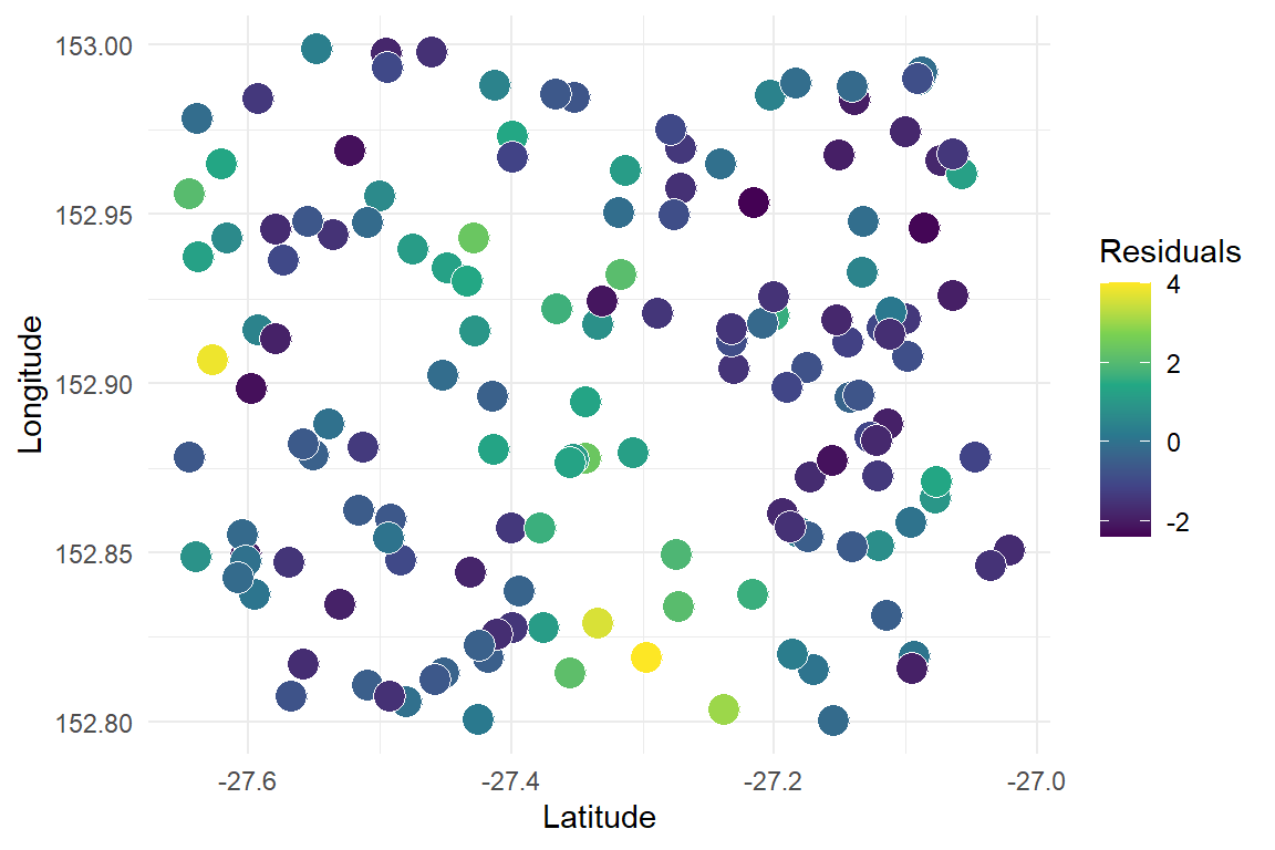
There are obvious spatial patterns in the model’s failures. We could compute a semivariogram to confirm but there is no need. We must proceed with a more appropriate model
Fit the geostatistical model to simulated data
Organise the data for Stan modelling into a list
model_data <- list(N = N,
                   # Distances matrix
                   distances = m,
                   # Number of covariates
                   K = 1,
                   # Covariate design matrix (for all points)
                   X = as.matrix(precip),
                   # Observed values of simulated outcomes
                   y = sim_y)
Condition the model on the observed data; some early warnings are likely as the sampler chooses among initial values for GP parameters, which can sometimes lead to covariance matrices that are not positive definite. Usually this resolves as the sampler moves through the warmup phase
fit <- cmd_mod$sample(data = model_data,
                      chains = 4,
                      iter_warmup = 500,
                      iter_sampling = 1000,
                      parallel_chains = 4,
                      refresh = 100)
Inspect sampler and convergence diagnostics. Any warnings of divergences or low energy should be taken seriously and inspected further. Fortunately our model fits without issue
fit$diagnostic_summary()
## $num_divergent
## [1] 0 0 0 0
##
## $num_max_treedepth
## [1] 0 0 0 0
##
## $ebfmi
## [1] 0.9313095 0.8574628 0.9105745 0.8735549
A quick summary of parameters of interest
fit$summary(c('rho', 'alpha', 'beta'))
## # A tibble: 3 × 10
##   variable  mean median     sd    mad    q5   q95  rhat ess_bulk ess_tail
##   <chr>    <dbl>  <dbl>  <dbl>  <dbl> <dbl> <dbl> <dbl>    <dbl>    <dbl>
## 1 rho      6.00   5.93  1.21   1.23   4.14  8.07   1.00     870.    1493.
## 2 alpha    0.795  0.779 0.150  0.133  0.587 1.07   1.00    1797.    1829.
## 3 beta[1]  0.366  0.364 0.0797 0.0811 0.240 0.499  1.00    6236.    2402.
These summaries are not that useful. Using posterior medians +/- credible intervals is never as informative as are visualisations of model parameters. Visualise posterior estimates for \(\alpha\) and overlay the true simulated value in black
hist(fit$draws("alpha", format = "draws_matrix"),
     col = c_mid_highlight, border = 'white', lwd = 2,
     main = '', yaxt = 'n', ylab = '', xlab = expression(alpha))
abline(v = alpha, lwd = 3.5, col = 'white')
abline(v = alpha, lwd = 3, col = 'black')
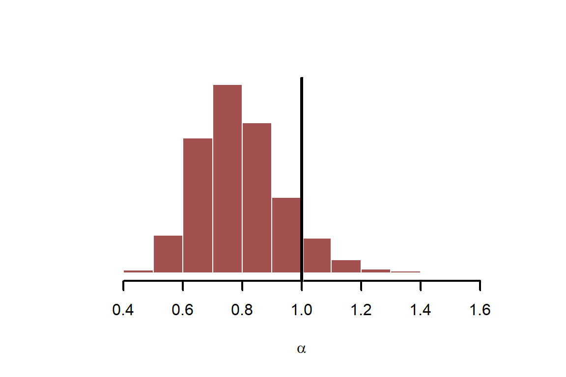
Repeat for the GP length scale parameter, \(\rho\)
hist(fit$draws("rho", format = "draws_matrix"),
     col = c_mid_highlight, border = 'white', lwd = 2,
     main = '', yaxt = 'n', ylab = '', xlab = expression(rho))
abline(v = rho, lwd = 3.5, col = 'white')
abline(v = rho, lwd = 3, col = 'black')
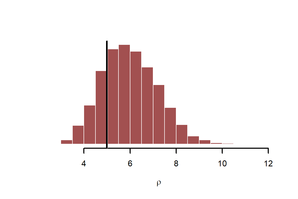
Now look at the regression coefficient for precipitation, \(\beta_{precip}\). You could (and generally should) also devise scenarios for prediction to help you better understand the model’s assumptions. But we will leave parameter inspection here for now
hist(fit$draws("beta[1]", format = "draws_matrix"),
     col = c_mid_highlight, border = 'white', lwd = 2,
     main = '', yaxt = 'n', ylab = '', xlab = expression(beta[precip]))
abline(v = beta_precip, lwd = 3.5, col = 'white')
abline(v = beta_precip, lwd = 3, col = 'black')
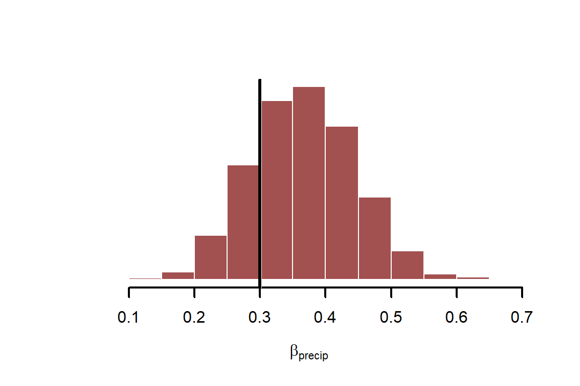
As with any regression, we should inspect residuals for any obvious discrepancies. Because our data are discrete counts bounded at zero, standard residuals aren’t helpful. We will use randomized quantile (Dunn-Smyth) residuals, which should be approximately standard normal in distribution. Don’t worry too much about the details, but I’m showing this function so the tutorial has complete code
ds_resids_pois = function(truth, fitted){
  na_obs <- is.na(truth)
  a_obs <- ppois(as.vector(truth[!na_obs]) - 1,
                 lambda = fitted[!na_obs])
  b_obs <- ppois(as.vector(truth[!na_obs]),
                 lambda = fitted[!na_obs])
  u_obs <- runif(n = length(fitted[!na_obs]),
                 min = pmin(a_obs, b_obs),
                 max = pmax(a_obs, b_obs))

  if(any(is.na(truth))){
    u_na <- runif(n = length(fitted[na_obs]),
                  min = 0, max = 1)
    u <- vector(length = length(truth))
    u[na_obs] <- u_na
    u[!na_obs] <- u_obs
  } else {
    u <- u_obs
  }
  dsres_out <- qnorm(u)
  dsres_out[is.infinite(dsres_out)] <- rnorm(length(which(is.infinite(dsres_out))))
  dsres_out
}
Calculate posterior retrodictions for the modeled observations. Notice how we use rpois to generate Poisson draws with the exact linear predictor that was used in our Stan model
beta_posterior <- fit$draws("beta[1]", format = "draws_matrix")
obs_gp_function_posterior <- fit$draws('gp_function',format = "draws_matrix")
preds <- matrix(NA, nrow = 1000, ncol = length(sim_y))
for(i in 1:1000){
  preds[i, ] <- rpois(length(sim_y),
                 lambda = exp((beta_posterior[i] * precip) +
                                          obs_gp_function_posterior[i,]))
}
Create a truth matrix for vectorised residual computation. This just replicates the observed values 1000 times so we don’t have to use a for loop to calculate residuals for all 1000 posterior predictions
truth_mat <- matrix(rep(sim_y, NROW(preds)),
                    nrow = NROW(preds),
                    byrow = TRUE)
Calculate posterior residuals
resids <- matrix(ds_resids_pois(truth = as.vector(truth_mat),
                                  fitted = as.vector(preds)),
                   nrow = NROW(preds))
As we saw above with the non-spatial model, a useful diagnostic is to plot residuals against observed values to see if there are any systematic discrepancies in observations vs predictions. We will plot 50 posterior draws of residuals because there is uncertainty in these parameters
plot(sim_y, resids[1,], ylim = range(resids), pch = 16,
     col = "#8F272720", bty = 'l',
     xlab = 'Observed count',
     ylab = 'Dunn-Smyth residual')
for(i in 2:50){
  points(sim_y, resids[i,], ylim = range(resids), pch = 16,
       col = "#8F272720")
}
box(bty = 'l', lwd = 2)
abline(h = 0, lwd = 3, col = 'white')
abline(h = 0, lwd = 2.5)
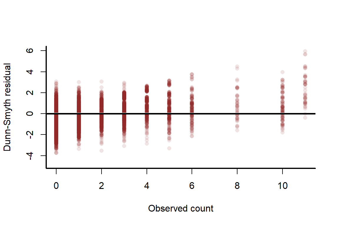
There is no alarming pattern here, though the model does tend to slightly under-predict large values. A normal Q-Q plot checks if there is any over- or under-dispersion that is not being captured by the model
qqnorm(resids[1,], pch = 16,
       bty = 'l', ylim = c(-6, 6), col = "#8F272730")
qqline(resids[1,], lwd = 0.5, col = '#80808040')
for(i in 2:50){
  qqline(resids[i,], lwd = 0.5, col = '#80808040')
}
for(i in 2:50){
  test <- qqnorm(resids[i,], plot = F)
  points(test$x, test$y, pch = 16, col = "#8F272730")
}
box(bty = 'l', lwd = 2)
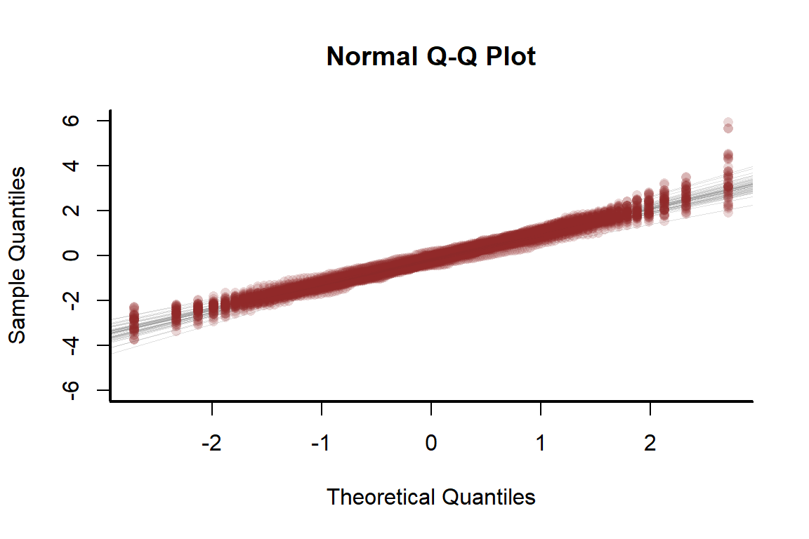
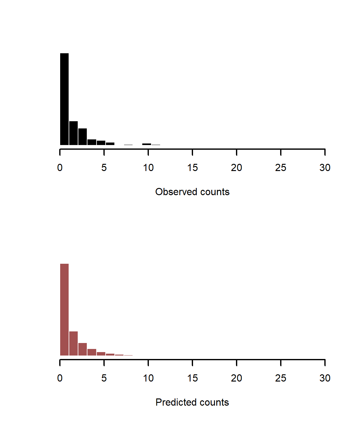
The points all fall nicely along the 1:1 lines, suggesting the model can simulate data that follow the distribution of the observed values. We can also plot histograms of observations vs predictions, as we did with the nonspatial model above
layout(matrix(1:2))
hist(sim_y, col = 'black',
     freq = F,
     breaks = seq(0, pmax(max(sim_y), max(preds)), length.out = 30),
     border = 'white', lwd = 2, xlab = 'Observed counts',
     yaxt = 'n', ylab = '', main = '')
hist(preds, col = c_mid_highlight,
     freq = F,
     breaks = seq(0, pmax(max(sim_y), max(preds)), length.out = 30),
     border = 'white', lwd = 2, xlab = 'Predicted counts',
     yaxt = 'n', ylab = '', main = '')
layout(1)
Inference
The model appears to simulate realistic-looking data. Moreover, all of our parameters were recovered well by the model. But what do these parameters actually mean? The GP parameters are best interpreted together, as they form the spatial covariance kernel. Those of you that have worked with variograms before will be used to visualising how semivariance decays over distance. Here we will visualise how covariance decays over distance. It is certainly worth visualising the posterior estimates for this kernel to see if the model captures the simulated covariance well. Define a function to compute the covariance kernel for each posterior draw
quad_kernel = function(rho, alpha, distances){
  covs <- alpha ^ 2 * exp(-0.5 * ((distances / rho) ^ 2))
}
Distances (in km) over which to compute the posterior kernel estimates
distances = seq(0, 100, length.out = 75)
Compute posterior kernels
kernels <- matrix(NA, nrow = 1000, ncol = length(distances))
rho_posterior <- fit$draws('rho', format = "df")$rho
alpha_posterior <- fit$draws('alpha', format = "df")$alpha
for(i in 1:1000){
  kernels[i,] <- quad_kernel(rho = rho_posterior[i],
                             alpha = alpha_posterior[i],
                             distances = distances)
}
Calculate posterior empirical quantiles for the kernel
probs <- c(0.05, 0.2, 0.3, 0.4, 0.5, 0.6, 0.7, 0.8, 0.95)
cred <- sapply(1:NCOL(kernels),
               function(n) quantile(kernels[,n],
                                    probs = probs))
Plot the estimated kernels and overlay the true simulated kernel in black
pred_vals <- distances
plot(1, xlim = c(0, 20), ylim = c(0, max(cred)), type = 'n',
     xlab = 'Distance (in km)', ylab = 'Covariance',
     bty = 'L')
box(bty = 'L', lwd = 2)
polygon(c(pred_vals, rev(pred_vals)), c(cred[1,], rev(cred[9,])),
        col = c_light, border = NA)
polygon(c(pred_vals, rev(pred_vals)), c(cred[2,], rev(cred[8,])),
        col = c_light_highlight, border = NA)
polygon(c(pred_vals, rev(pred_vals)), c(cred[3,], rev(cred[7,])),
        col = c_mid, border = NA)
polygon(c(pred_vals, rev(pred_vals)), c(cred[4,], rev(cred[6,])),
        col = c_mid_highlight, border = NA)
lines(pred_vals, cred[5,], col = c_dark, lwd = 2.5)

# Overlay the true simulated kernel
true_kernel <- quad_kernel(rho = rho,
                           alpha = alpha,
                           distances = distances)
lines(pred_vals,
      true_kernel, lwd = 3.5, col = 'white')
lines(pred_vals,
      true_kernel, lwd = 3, col = 'black')
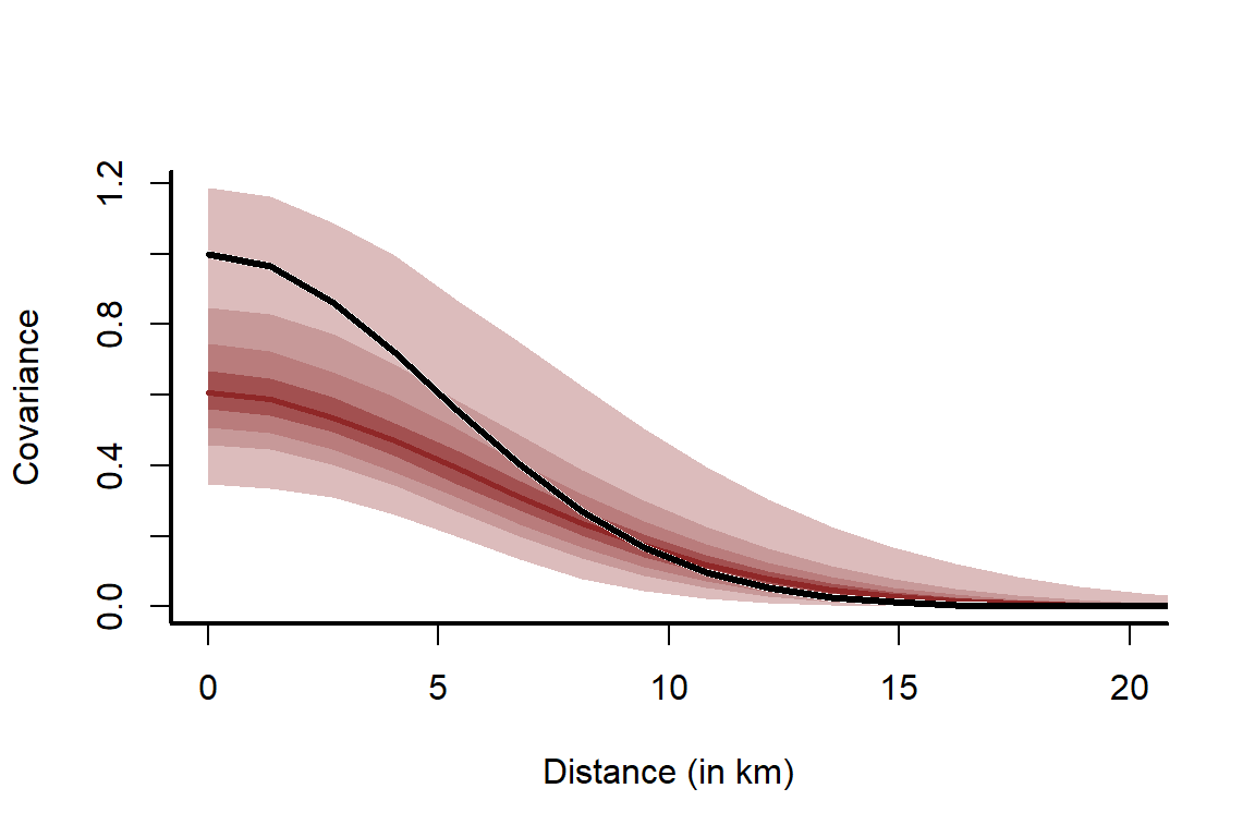
This plot clearly shows that locations close together (further left on the x-axis) exhibit stronger covariance. The model does a reasonable job of estimating the true simulated kernel, though it does over-smooth a bit (because it slightly overestimates \(\rho\)). We can’t expect perfection when we used a noisy observation process (Poisson draws) and only 150 points. This is why it is so important to quantify our uncertainty in model parameters / functions.
Prediction
A common goal in spatial modeling is to generate smoothed predictions for unsampled locations. We want our predictions to respect the spatial patterns that our model has estimated. We also want predictions to respect uncertainty in model parameters. To generate predictions, we have to take draws from the appropriate multivariate normal distribution. First, define a function to calculate distances (in km) among pairs of points
calc_point_distances = function(coordinates, coordinates2){
  if(missing(coordinates2)){
    distances <- pointDistance(coordinates, lonlat = TRUE)
    distances[upper.tri(distances)] = t(distances)[upper.tri(distances)]
  } else {
    distances <- pointDistance(coordinates, coordinates2, lonlat = TRUE)
  }

  # Convert meters distance to kilometers
  distances <- distances / 1000

  return(distances)
}
Next, we need a function to predict from a GP for a grid of spatial points. This function takes the modeled datapoints (i.e. the 150 that we used to train the model) and works out how to propagate the Gaussian Process from the modeled datapoints to a new set of prediction points. Don’t worry if you don’t understand the linear algebra. Just understand that we cannot predict for a new set of points without calculating the cross-covariance between fitted points and prediction points
predict_gp <- function(alpha, rho, obs_gp_function,
                       obs_distances, pred_distances,
                       obs_to_pred_distances){

  # Estimated covariance kernel for the fitted points
  K_obs <- alpha ^ 2 * exp(-0.5 * ((obs_distances / rho) ^ 2)) +
    diag(1e-4, dim(obs_distances)[1])

  # Cross-covariance between prediction points and fitted points
  K_new <- alpha ^ 2 * exp(-0.5 * ((obs_to_pred_distances / rho) ^ 2))

  # Estimated covariance kernel for prediction points
  K_star <- alpha ^ 2 * exp(-0.5 * ((pred_distances / rho) ^ 2)) +
    diag(1e-4, dim(pred_distances)[1])

  # Estimated mean for prediction points
  t(K_new) %*% solve(K_obs, obs_gp_function) +
    # One realisation of uncertainty for prediction points
    MASS::mvrnorm(1, mu = rep(0, dim(pred_distances)[1]),
                  Sigma = K_star - t(K_new) %*% solve(K_obs, K_new))
}
Next generate a spatial grid of 1000 points covering the extent of the simulated study area
pred_grid <- as.data.frame(makegrid(as(raster::extent(152.8, 153, -27.65, -27),
                                       'SpatialPolygons'), n = 1000))
colnames(pred_grid) <- c('Longitude', 'Latitude')
Calculate distances among fitted and prediction points (in km)
obs_distances <- calc_point_distances(coordinates = coords)
pred_distances <- calc_point_distances(coordinates = pred_grid)
obs_to_pred_distances <- calc_point_distances(coords, pred_grid)
Extract posterior estimates for the latent GP function that applied to the in-sample (fitted) observations
obs_gp_function_posterior <- fit$draws('gp_function',format = "df")[,1:N]
## Warning: Dropping 'draws_df' class as required metadata was removed.
Generate latent GP predictions using 5 posterior draws. This computation can be sped up by parallelising the operation later on, but for now we just have to sit and wait. For a real analysis, we’d want at least 1000 estimates so we could accurately quantify our uncertainty
gp_preds <- matrix(NA, nrow = 5, ncol = NROW(pred_grid))
for(i in 1:NROW(gp_preds)){
  cat('Processing posterior draw', i, 'of 5...\n')
  gp_preds[i,] <- predict_gp(obs_distances = obs_distances,
                             pred_distances = pred_distances,
                             obs_to_pred_distances = obs_to_pred_distances,
                             obs_gp_function = as.vector(as.matrix(obs_gp_function_posterior[i,])),
                             alpha = alpha_posterior[i],
                             rho = rho_posterior[i])
}
## Processing posterior draw 1 of 5...
## Processing posterior draw 2 of 5...
## Processing posterior draw 3 of 5...
## Processing posterior draw 4 of 5...
## Processing posterior draw 5 of 5...
Plot the posterior mean spatial GP predictions just for a quick visualisation
grid2 <- data.frame(pred_grid)
grid2$preds <- colMeans(gp_preds)
colnames(grid2) <- c('Longitude', 'Latitude', 'GP_function')
ggplot(grid2,
       aes(x = Latitude, y = Longitude, fill = GP_function)) +
  geom_point(shape = 21, col = 'white', size = 4) +

  # Highlight the original simulated points as larger circles
  # to ensure the spatial kriging makes sense
  geom_point(data = data.frame(sim_y = sim_y,
                        GP = sim_gp,
                        Longitude = lon,
                        Latitude = lat),
             aes(x = Latitude, y = Longitude, fill = GP),
             size = 5, shape = 21, col = 'black') +
  scale_fill_continuous(type = "viridis") +
  theme_minimal()
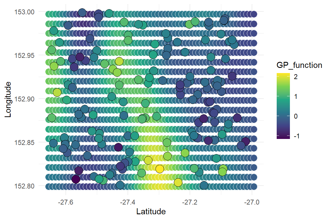
For complete predictions, we would need the covariate values (i.e. precipitation) at all of the spatial locations. The predictions would be just as fast, we would simply need to take posterior draws of \(\beta_{precip}\), multiply them by the covariate values at each point, then add those with the GP estimates to form the linear predictor for \(log(\lambda)\). We could then use rpois(exp(prediction)) to draw a Poisson realisation for each prediction point that satisfies \(Poisson(\lambda)\)