Phylogenetic smoothing using mgcv

By Nicholas Clark in rstats mgcv

February 24, 2024

I have been highly interested in multivariate time series modeling for the last few years and have spent a lot of time working out how to use hierarchical GAMs to tackle many of the questions I’m interested in. As you may already know, GAMs afford us a huge amount of flexibility to address nonlinear associations in ecological models ( see this paper by Pedersen et al for some more context). I have done quite a bit of work to extend these models to also capture complex dynamic processes, which are available in my mvgam R package.

But I have recently become aware that it is possible to use phylogenetic or functional information to regularize these hierarchical functions. This works by taking advantage of the hugely flexible mrf basis that is provided in mgcv (see ?mgcv::mrf for details). This basis allows users to provide their own penalty matrices, which will act as a prior precision for the basis coefficients when estimating the model. By providing the right kind of penalty matrix, for example one that is constructed from a phylogenetic tree or functional dendrogram, we can force the model to regularize species’ nonlinear effects toward those from their most closely related neighbours. This is an incredible advance that opens many new possibilities for asking targeted questions about niche conservatism, trait evolution, functional redundancy and a whole host of other directions. A very basic example of how this can be done in mgcv is presented here.

Environment setup

Load libraries necessary for data manipulation and modeling

library(ape)
library(mgcv)
library(mvnfast)
library(ggplot2)
library(dplyr)
library(MRFtools) # devtools::install_github("eric-pedersen/MRFtools")

A utility function to simulate from a squared exponential Gaussian Process, which we will use to create species’ nonlinear temporal trends

sim_gp = function(N, alpha, rho){
  Sigma <- alpha ^ 2 *
    exp(-0.5 * ((outer(1:N, 1:N, "-") / rho) ^ 2)) +
    diag(1e-9, N)
  mvnfast::rmvn(1,
                mu = rep(0, N),
                sigma = Sigma)[1,]
}

Phylogenetically structured trends

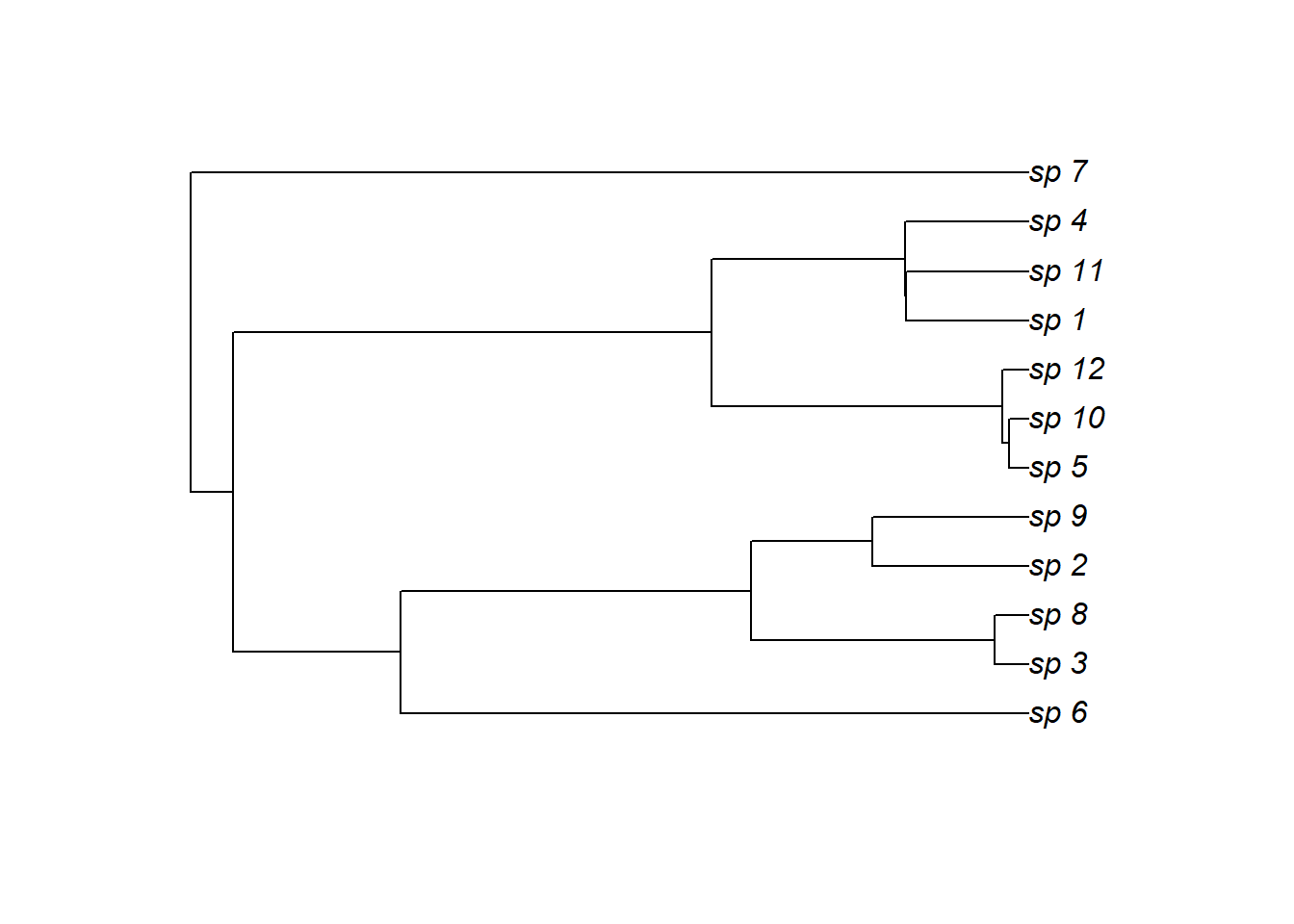
Simulate a random phylogenetic tree to inform species’ relationships

N_species <- 12
tree <- rcoal(N_species, tip.label = paste0('sp_', 1:N_species))
species_names <- tree$tip.label
plot(tree)

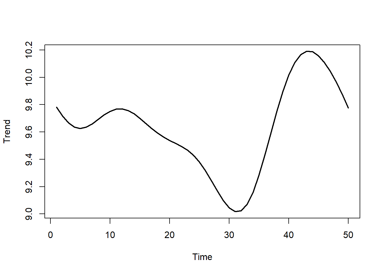
Now simulate a ‘shared’ nonlinear temporal trend, which will anchor each species’ trend

N <- 50
shared <- sim_gp(N, alpha = 1, rho = 8) + 10
plot(shared, type = 'l', lwd = 2, xlab = 'Time', ylab = 'Trend')

Next we construct the phylogenetically-informed trends. In this example, each species’ actual trend is a perturbation of the shared trend, whereby the final trend is a weighted sum of the shared trend and two other GP trends. Because the weights are simulated using phylogenetic information (using the rTraitCont() function from the ape library), this process allows us to construct smooth trends that will hopefully capture the property we’re after, i.e. that more closely related species will have more similar functional shapes

warp1 <- sim_gp(N, alpha = 2, rho = 20) + 10
warp2 <- sim_gp(N, alpha = 2, rho = 20) + 10
weights1 <- as.vector(scale(rTraitCont(tree)))
weights2 <- as.vector(scale(rTraitCont(tree)))

Create the trends for each species and take noisy observations. For the third and seventh species, we set observations to NA so we can test if the model is able to recover their trends. Store all necessary data in a data.frame

dat <- do.call(rbind, 
               lapply(seq_len(N_species),
                      function(i){
                        sp_trend <- warp1 * weights1[i] + 
                          warp2 * weights2[i] + shared
                        obs <- rnorm(N, 
                                     mean = as.vector(scale(sp_trend)),
                                     sd = 0.35)
                        if(i %in% c(3, 7)){
                          weight <- 0
                          obs <- NA
                        } else {
                          weight <- 1
                        }
                        data.frame(species = species_names[i],
                                   weight = weight,
                                   time = 1:N,
                                   truth = as.vector(scale(sp_trend)),
                                   y = obs)
                      }))
dat$species <- factor(dat$species, levels = species_names)

We’ll also leave out the last 5 observations for each species so we can see how well (or how poorly) the trends extrapolate, though this isn’t the primary focus of the example

dat %>%
  dplyr::mutate(y = dplyr::case_when(
    time <= N-5 ~ y,
    time > N-5 ~ NA,
    TRUE ~ y
  )) -> dat

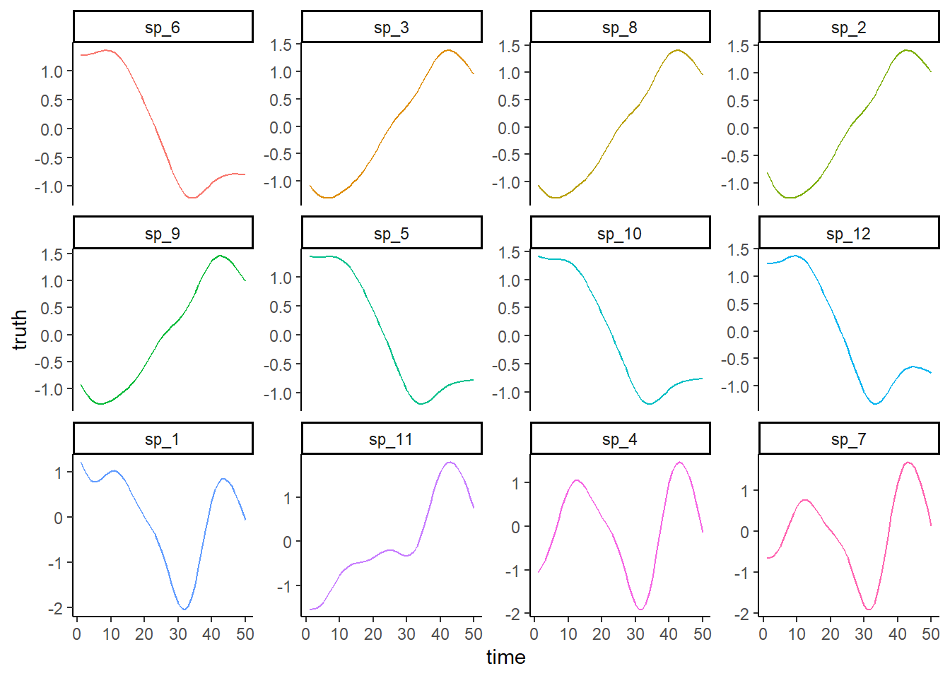
Data visualisation

Plot the true simulated trends for each species

ggplot(dat, aes(x = time, y = truth, col = species)) +
  geom_line() +
  facet_wrap(~species, scales = 'free_y') + 
  theme_classic() +
  theme(legend.position = 'none')

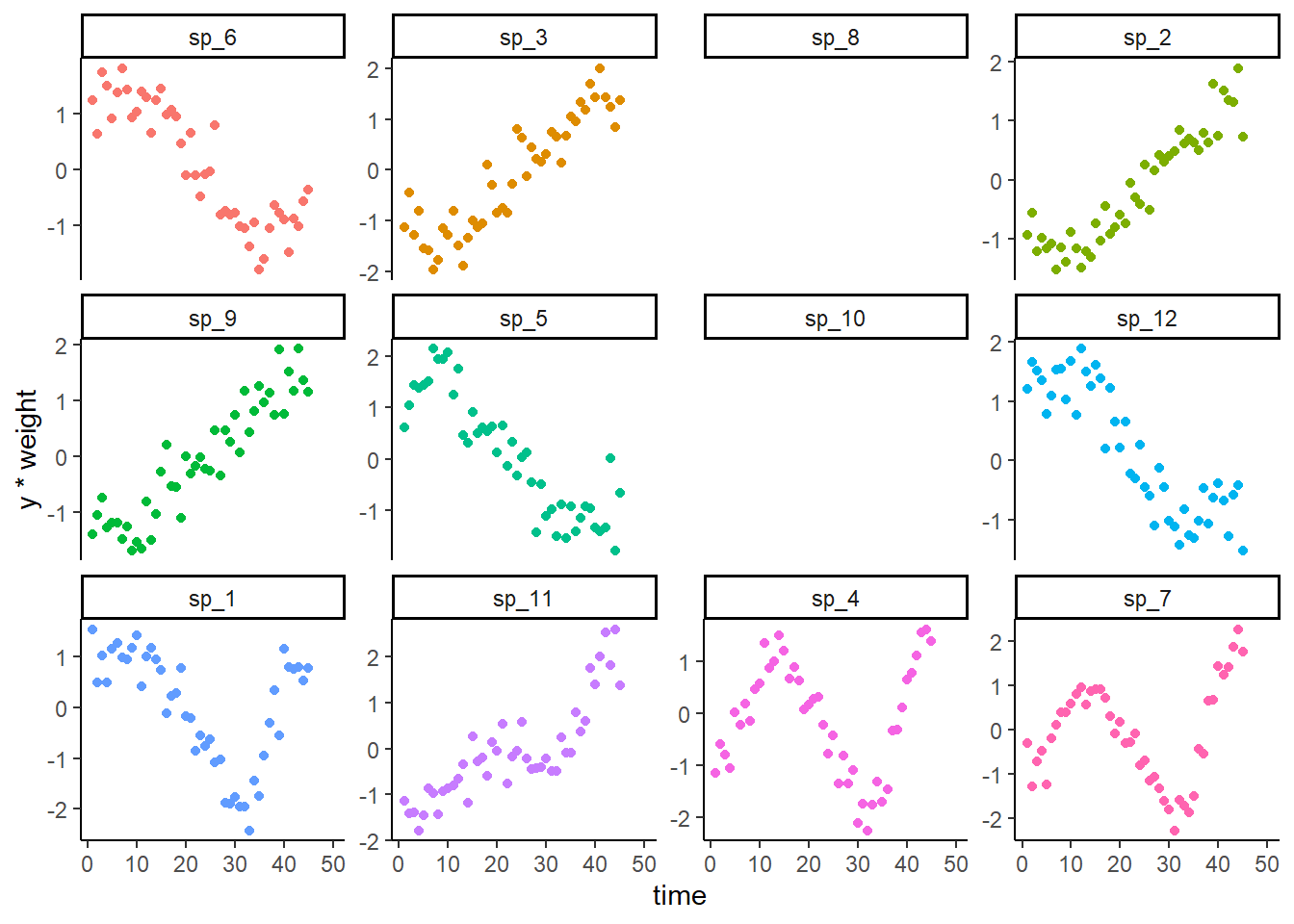
Simulating species' nonlinear time trends using phylogenetic relationships.

Plot the noisy observations (noting that all obs are missing for two species)

ggplot(dat, aes(x = time, y = y*weight, col = species)) +
  geom_point() +
  facet_wrap(~species, scales = 'free_y') + 
  theme_classic() +
  theme(legend.position = 'none')

## Warning: Removed 150 rows containing missing values or values outside the scale range
## (`geom_point()`).

Simulating noisy observations of species' nonlinear time trends using phylogenetic relationships.

Model setup

Create the MRF penalty matrix using the phylogenetic precision matrix

omega <- solve(vcv(tree))

Now add an MRF penalty that forces the temporal trend to evolve as a Random Walk using utilities provided by Pedersen et al’s MRFtools package. This requires that we have a factor variable for time in our data, and we should ensure the levels of this time_factor go as high as we would potentially like to forecast. Note that this package can also create the phylogenetic penalty but I feel it is better to show these steps explicitly for this example.

rw_penalty <- mrf_penalty(object = 1:max(dat$time), 
                          type = 'linear')
dat$time_factor <- factor(1:max(dat$time))

Fit a GAM using a tensor product of the RW MRF basis and the phylogenetic MRF basis. We also use a ‘shared’ smooth of time so that the phylogenetic smooths are estimated as deviations around this shared smooth. Set drop.unused.levels = FALSE to ensure there are no errors because of the extra species and times in the penalty matrices

mod <- gam(y ~ s(time, k = 10) + 
               te(time_factor, species, 
                  bs = c("mrf", "mrf"),
                  k = c(8, N_species),
                  xt = list(list(penalty = rw_penalty), 
                            list(penalty = omega))),
           data = dat,
           drop.unused.levels = FALSE,
           method = "REML")
summary(mod)

## 
## Family: gaussian 
## Link function: identity 
## 
## Formula:
## y ~ s(time, k = 10) + te(time_factor, species, bs = c("mrf", 
##     "mrf"), k = c(8, N_species), xt = list(list(penalty = rw_penalty), 
##     list(penalty = omega)))
## 
## Parametric coefficients:
##             Estimate Std. Error t value Pr(>|t|)  
## (Intercept) -0.03469    0.01665  -2.084   0.0378 *
## ---
## Signif. codes:  0 '***' 0.001 '**' 0.01 '*' 0.05 '.' 0.1 ' ' 1
## 
## Approximate significance of smooth terms:
##                            edf Ref.df      F p-value    
## s(time)                  6.011  6.576  2.239  0.0281 *  
## te(time_factor,species) 67.709 79.000 39.045  <2e-16 ***
## ---
## Signif. codes:  0 '***' 0.001 '**' 0.01 '*' 0.05 '.' 0.1 ' ' 1
## 
## R-sq.(adj) =  0.892   Deviance explained =   91%
## -REML = 291.42  Scale est. = 0.12468   n = 450

Predictions and evaluation

Calculate predictions from the model for the full dataset (including the missing species) and overlay the actual true simulated trends as black points. Did the model successfully estimate the missing species’ temporal trend?

preds <- predict(mod, newdata = dat, type = 'response', se = TRUE)
dat$pred <- preds$fit
dat$upper <- preds$fit + 1.96*preds$se.fit
dat$lower <- preds$fit - 1.96*preds$se.fit
ggplot(dat, aes(x = time, y = pred, col = species)) +
  geom_point(aes(y = truth), col = 'black') +
  geom_line(linewidth = 1, alpha = 0.6) +
  geom_ribbon(aes(ymin = lower, ymax = upper, fill = species),
              alpha = 0.3, col = NA) +
  facet_wrap(~species, scales = 'free_y') + 
  theme_classic() +
  theme(legend.position = 'none')

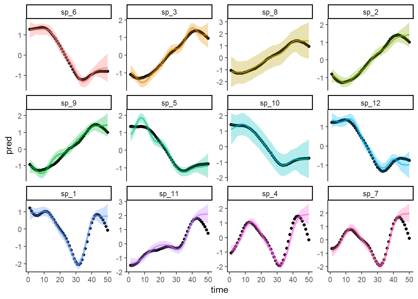
Predicting species' nonlinear time trends using Hierarchical Generalized Additive Models with phylogenetic smooths.

Hot Damn it worked! But could we recover these missing trends without the information provided in the phylogenetic structure? Fit a second GAM that uses a similar hierarchical smooth of time, but in this case the deviations around the shared smooth do not have any phylogenetic information to leverage

mod2 <- gam(y ~ s(time, k = 10) +
              s(time, species, bs = 'fs', k = 8),
           data = dat,
           method = "REML",
           drop.unused.levels = FALSE)

## Warning in gam.side(sm, X, tol = .Machine$double.eps^0.5): model has repeated
## 1-d smooths of same variable.

summary(mod2)

## 
## Family: gaussian 
## Link function: identity 
## 
## Formula:
## y ~ s(time, k = 10) + s(time, species, bs = "fs", k = 8)
## 
## Parametric coefficients:
##             Estimate Std. Error t value Pr(>|t|)
## (Intercept) -0.03469    0.03615   -0.96    0.338
## 
## Approximate significance of smooth terms:
##                    edf Ref.df     F  p-value    
## s(time)          7.668  8.285  5.13 3.06e-06 ***
## s(time,species) 56.239 78.000 38.27  < 2e-16 ***
## ---
## Signif. codes:  0 '***' 0.001 '**' 0.01 '*' 0.05 '.' 0.1 ' ' 1
## 
## R-sq.(adj) =  0.889   Deviance explained = 90.5%
## -REML = 285.82  Scale est. = 0.12807   n = 450

Now predict from the non-phylogenetic model

preds <- predict(mod2, newdata = dat, type = 'response', se = TRUE)
dat$pred <- preds$fit
dat$upper <- preds$fit + 1.96*preds$se.fit
dat$lower <- preds$fit - 1.96*preds$se.fit
ggplot(dat, aes(x = time, y = pred, col = species)) +
  geom_point(aes(y = truth), col = 'black') +
  geom_line(linewidth = 1, alpha = 0.6) +
  geom_ribbon(aes(ymin = lower, ymax = upper, fill = species),
              alpha = 0.3, col = NA) +
  facet_wrap(~species, scales = 'free_y') + 
  theme_classic() +
  theme(legend.position = 'none')

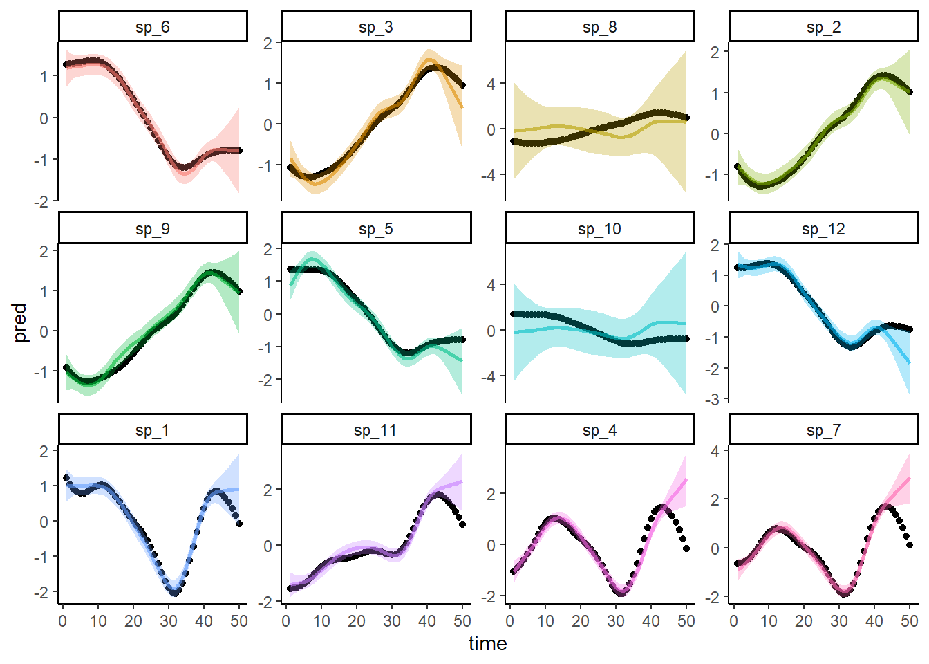
Predicting species' nonlinear time trends using hierarchical Generalized Additive Models.

Predictions from this model draw from the ‘average’ smooth, rather than leveraging phylogenetic information, to predict the trends for the missing species. So the predictions for both missing species are identical. Obviously we can tell by eye that the predictions are worse than those from the phylogenetic model. But we could use Continuous Rank Probability Scores for each model’s predictions to quantify how much worse

Environment setup

Phylogenetically structured trends

Data visualisation

Model setup

Predictions and evaluation

Further reading