Using Stan for logistic regressions with detection error
By Nicholas Clark in stan simulation
March 10, 2024
Required libraries
cmdstanr
Purpose and model introduction
This script simulates binary observations of an imperfectly observed data generating process (i.e. our measurements are made with error). It also provides Stan code for estimating parameters of the model in a Bayesian framework. The true infection status \(z\) is assumed to be drawn from a Bernoulli distribution with probability \(p\):
$$z\sim \text{Bernoulli}(p)$$
A linear predictor is modeled on the \(logit\) scale to capture effects of covariates on \(p\):
$$logit(p)={\alpha} + {\beta}*\boldsymbol{X}$$
\(\alpha\) is the intercept representing average infection probability when all predictor variables are set to their means, and \(\beta\) is the set of regression coefficients that describe associations between predictor variables in the model design matrix \(\boldsymbol{X}\) and \(logit(p)\). Unfortunately, as is the case in most diagnostic test scenarios, our measurements are made with error. A classic example would be a Kato Katz faecal smear to detect eggs of soil-transmitted helminths. We know these tests are not perfect. It is easy to miss a parasite egg when the smear quality is low. Or when parasite eggs are not being shed. Or because eggs are damn small and hard to see. Assume \(\hat{SN}\) is our test’s sensitivity (the proportion of subjects with the condition that tend to have a positive test) and \(\hat{SP}\) is the test’s specificity (the proportion of subjects without the condition that tend to have a negative test). Observations \(\boldsymbol{Y}\) are assumed to be conditional on the latent, unobserved true infection status \(z\) through the following set of equations:
$$\boldsymbol{Y}\sim \text{Bernoulli}(\hat{SN}),~if~~z~= 1$$
$$\boldsymbol{Y}\sim \text{Bernoulli}(1 - \hat{SP}),~if~~z~= 0$$
Ignoring this detection error is bad. It can bias our estimates and lead to incorrect inferences. But there are several challenges with estimating such a model. First, we often do not know with precision what the test’s specificity and sensitivity are. So we need to estimate them. The second issue is that the \(z\) represent latent discrete parameters. We do not know what the true infection status is. We could try to sample it, but it turns out that
sampling these latent values is problematic for advanced MCMC routines such as Stan’s Hamiltonian Monte Carlo algorithm. Other types of samplers (i.e. Gibbs or Metropolis Hastings, like those used in JAGS or BUGS) will allow latent discrete parameters, but they are not efficient. Fortunately, probability theory tells us how we can account for the possibility that the true status \(z\) was either a 1 or a 0 using a
marginal likelihood. The unconditional probability of the observed infection status \(\boldsymbol{Y}\) is the sum of the probability in each unknown state (truly infected or truly uninfected) times the chance of being in each unknown state. This actually leads to better estimates because the expectation at all possible values is being used, rather than being estimated by sampling a latent discrete parameter.
Define the joint probabilistic model
First we will define the Stan model code for estimating parameters under the model outlined above. This code uses a logical flag to allow us to tell the sampler whether or not to account for detection error. This will be useful for investigating the consequences of model misspecification.
model_code <-
"data {
  int<lower=0> N; // number of observations
  int<lower=0> P; // number of (standardised) predictor variables
  array[N] int<lower=0, upper=1> y; // binary infection observations
  matrix[N, P] x; // predictor design matrix
  real<lower=-1,upper=1> sensitivity_prior; // inerpretable prior on sensitivity
  real<lower=-1,upper=1> specificity_prior; // inerpretable prior on specificity
  int<lower=0,upper=1> estimate_accuracy; // logical (include detection error or not)
}

transformed data {
  // Convert diagnostic hyperpriors into values to feed to the dirichlet
  real<lower=0> sens_hyp;
  real<lower=0> spec_hyp;
  real<lower=0> remainder_hyp;
  sens_hyp = 1 / exp(sensitivity_prior);
  spec_hyp = 1 / exp(specificity_prior);
  remainder_hyp = exp(sensitivity_prior) + exp(specificity_prior);

  // QR decomposition to deal with (possibly) correlated predictor variables
  // https://betanalpha.github.io/assets/case_studies/qr_regression.html
  matrix[N, P] Q_ast;
  matrix[P, P] R_ast;
  matrix[P, P] R_ast_inverse;
  Q_ast = qr_thin_Q(x) * sqrt(N - 1);
  R_ast = qr_thin_R(x) / sqrt(N - 1);
  R_ast_inverse = inverse(R_ast);
}

parameters {
  vector[P] theta; // QR decomposed regression coefficients
  real alpha; // intercept coefficient
  vector<lower=1>[3] theta_acc; // hyperprior for test accuracy
  simplex[3] accuracy; // sum-to-1 constraint for misclassification error
}

transformed parameters {
  // test sensitivity and specificity
  real<lower=0, upper=1> sens;
  real<lower=0, upper=1> spec;

  // set both to 1 if we don't want to estimate detection error
  if (estimate_accuracy)
   sens = 1 - accuracy[1];
  else
   sens = 1;

  if (estimate_accuracy)
   spec = 1 - accuracy[2];
  else
   spec = 1;

  // linear predictor for the logistic regression; here we can also include
  // terms for spatial, temporal, and spatiotemporal effects; some examples found here:
  // https://mc-stan.org/docs/stan-users-guide/fit-gp.html
  // https://betanalpha.github.io/assets/case_studies/gp_part1/part1.html#1_gaussian_processes
  // https://github.com/nicholasjclark/mvgam
  vector[N] logit_z = alpha + Q_ast * theta;
}

model {
  // informative hyperpriors on 1 - sensitivity and 1 - specificity
  theta_acc[1] ~ normal(sens_hyp, 0.25);
  theta_acc[2] ~ normal(spec_hyp, 0.25);
  // hyperprior for sum-to-one constraint
  theta_acc[3] ~ normal(remainder_hyp, 0.25);
  accuracy ~ dirichlet(theta_acc);

  // priors for regression coefficients
  // we assume the disease is a bit rare, so use an appropriate
  // prior on the intercept alpha
  alpha ~ normal(-0.75, 1);
  theta ~ std_normal();

  // marginal Bernoulli likelihood
  // the unconditional probability of the observed infection status is the sum of the
  // probability in each unknown state (truly infected or truly uninfected)
  // times the chance of being in each unknown state

  // for each observation, we calculate the probability that the 'true' status was a 1
  // and the probability that the 'true' status was a 0. Summing these probabilities on
  // the log scale is the same as multiplying them on the untransformed scale; this
  // allows us to average over (i.e. marginalise out) the latent infection status
  for (n in 1:N) {
    target += log_sum_exp(bernoulli_lpmf(y[n] | sens) + bernoulli_logit_lpmf(1 | logit_z[n]),
                          bernoulli_lpmf(1 - y[n] | spec) + bernoulli_logit_lpmf(0 | logit_z[n]));
  }
}

generated quantities {
  vector<lower=0, upper=1>[N] prob;
  array[N] int<lower=0, upper=1> ypred;
  vector[P] beta;

  // compute predicted infection probabilities (i.e. posterior expectations)
  // for each individual in the dataset
  for (n in 1:N) {
    prob[n] = softmax([bernoulli_lpmf(y[n] | sens) + bernoulli_logit_lpmf(1 | logit_z[n]),
                       bernoulli_lpmf(1 - y[n] | spec) + bernoulli_logit_lpmf(0 | logit_z[n])]')[1];
  }

  // compute predicted infection statuses (i.e. posterior predictions)
  // for each individual in the dataset
  ypred = bernoulli_rng(prob);

  // compute the regression coefficients for the original
  // (back-transformed) predictor variables
  beta = R_ast_inverse * theta;
}"
There is a lot going on in this model. It accepts interpretable hyperprior information for the test diagnostics (more on that below). It also uses a
QR decomposition to handle possible colinearity among predictors. And of course, it marginalises over discrete latent infection status. Details of each of these procedures are not the main aim of this tutorial, but please see the relevant hyperlinks for more information. Load cmdstanr and compile the model to C++ code. See
information here for troubleshooting advice when installing Stan and Cmdstan
library(cmdstanr)
mod <- cmdstan_model(write_stan_file(model_code),
                        stanc_options = list('canonicalize=deprecations,braces,parentheses'))
Simulate data
Now that the model is defined in Stan language, we need to simulate data to explore the model. Here we define a function to generate simulated binary outcomes with user-specific sensitivity and specificity. This function was modified from a very helpful
Stan discourse post
sim_det_error <- function(n = 200, # sample size
                          alpha = -0.5, # intercept (on logit scale)
                          p = 2, # number of predictors
                          sn = 0.85, # sensitivity of test
                          sp = 0.7) # specificity of test
  {

  # generate random predictors; note that predictors should be mean-centred
  # prior to modelling for the QR decomposition to be effective
  x <- rnorm(n*p, mean = 0, sd = 1)
  x <- matrix(x, nrow = n, ncol = p)
  colnames(x) <- paste0('predictor_', 1:p)

  # generate beta coefficients
  c <- rnorm(p, mean = 0, sd = 1)

  # design matrix and linear predictor
  x_design <- cbind(rep(1, n), x)
  c_full <- c(alpha, c)
  odds <- rowSums(sweep(x_design, 2, c_full, FUN = "*"))

  # convert linear predictor to the probability scale (logit link)
  pr <- 1 / (1 + exp(-odds))

  # generate true infection data
  truth <- rbinom(n = n, size = 1, prob = pr)

  # generate observed data with imperfect detection
  y <- integer(n)
  for ( i in 1:n ) {
    y[i] <- ifelse(truth[i] == 1, rbinom(n = 1, size = 1, prob = sn),
                     rbinom(n = 1, size = 1, prob = 1 - sp))
  }

  return(list(N = n,
              P = p,
              y = y,
              x = x,
              true_status = truth,
              true_sens = sn,
              true_spec = sp,
              true_alpha = alpha,
              true_betas = c))
}
Simulate some data with two predictors. Here sensitivity ($\hat{SN}$) = 0.75 and specificity ($\hat{SP}$) = 0.85. Again, sensitivity is a measure of how well a test can identify true positives and specificity is a measure of how well a test can identify true negatives. These values are not unreasonable given our knowledge of how difficult it can be to detect parasite eggs in faecal smears
dat <- sim_det_error(n = 250, alpha = -0.85,
                     p = 2, sn = 0.75, sp = 0.85)
The true (latent) prevalence is
sum(dat$true_status) / length(dat$true_status)
## [1] 0.324
The observed prevalence is
sum(dat$y) / length(dat$y)
## [1] 0.316
Add interpretable ‘prior’ information about test accuracy to the data, which will be used to structure the prior distributions for test sensitivity and specificity. Here, we use a scale of -1 to 1 to define any prior information we may have about performance of a diagnostic test. A score of -1 means we are fairly certain the test is bad (low accuracy). A score of 1 implies we are fairly certain the test is good. A score of 0 means we are uncertain. Let’s assume the test gives reasonable accuracy because it is a commercial diagnostic.
dat$sensitivity_prior <- 0.3
dat$specificity_prior <- 0.3
Fit competing models
We can assess whether it is problematic to ignore detection error when fitting models. We’ll do this by starting with a basic logistic regression that ignores this error. To do this, we include a logical flag to tell the sampler not to include detection error
dat$estimate_accuracy <- 0
Now condition the model on the observed data using Stan with the CmdStan backend
fit_noerror <- mod$sample(
  data = dat,
  chains = 4,
  parallel_chains = 4,
  refresh = 100)
Next we fit an equivalent model that does estimate detection error (i.e. we change the logical flag for estimate_accuracy from 0 to 1)
dat$estimate_accuracy <- 1
fit_error <- mod$sample(
  data = dat,
  chains = 4,
  parallel_chains = 4,
  refresh = 100)
Inspect sampler and convergence diagnostics. Any warnings of divergences or low energy should be taken seriously and inspected further. Fortunately our models fit without issue
fit_noerror$diagnostic_summary()
## $num_divergent
## [1] 0 0 0 0
##
## $num_max_treedepth
## [1] 0 0 0 0
##
## $ebfmi
## [1] 0.9662539 1.0130262 0.9480790 0.9575079
fit_error$diagnostic_summary()
## $num_divergent
## [1] 0 0 0 0
##
## $num_max_treedepth
## [1] 0 0 0 0
##
## $ebfmi
## [1] 0.9283966 0.8561576 0.8213387 0.8475217
Compute the usual MCMC summaries, which show that the Hamiltonian Monte Carlo chains have converged nicely
fit_noerror$summary(variables = c("alpha", "beta"))
## # A tibble: 3 × 10
##   variable   mean median    sd   mad     q5    q95  rhat ess_bulk ess_tail
##   <chr>     <dbl>  <dbl> <dbl> <dbl>  <dbl>  <dbl> <dbl>    <dbl>    <dbl>
## 1 alpha    -0.868 -0.865 0.142 0.143 -1.11  -0.640  1.00    4238.    2562.
## 2 beta[1]   0.345  0.346 0.150 0.147  0.100  0.591  1.00    3803.    3122.
## 3 beta[2]   0.389  0.388 0.148 0.150  0.149  0.634  1.00    4341.    2867.
fit_error$summary(variables = c("alpha", "beta", "sens", "spec"))
## # A tibble: 5 × 10
##   variable   mean median     sd    mad     q5     q95  rhat ess_bulk ess_tail
##   <chr>     <dbl>  <dbl>  <dbl>  <dbl>  <dbl>   <dbl> <dbl>    <dbl>    <dbl>
## 1 alpha    -1.18  -1.16  0.679  0.673  -2.34  -0.0840  1.00    2060.    2461.
## 2 beta[1]   0.799  0.722 0.466  0.400   0.199  1.65    1.00    1893.    1484.
## 3 beta[2]   0.814  0.759 0.403  0.375   0.262  1.55    1.00    1950.    1799.
## 4 sens      0.721  0.720 0.152  0.181   0.474  0.962   1.00    1456.    1391.
## 5 spec      0.848  0.844 0.0648 0.0674  0.747  0.965   1.00    1542.    1056.
Inference
Visualising the estimated coefficients for each of the models will allow us to ask whether ignoring detection error leads to biased inferences. First, define some colours for nice plots
c_light <- c("#DCBCBC")
c_light_highlight <- c("#C79999")
c_mid <- c("#B97C7C")
c_mid_highlight <- c("#A25050")
c_dark <- c("#8F2727")
c_dark_highlight <- c("#7C0000")
Plot the estimates for the intercept parameter \(\alpha\) and overlay the true simulated value in black
alphas_noerror <- fit_noerror$draws("alpha", format = "draws_matrix")
alphas_error <- fit_error$draws("alpha", format = "draws_matrix")

layout(matrix(1:2, ncol = 1))
par(mar = c(4, 1, 1.5, 1))
hist(alphas_noerror,
     col = 'grey', border = 'white', lwd = 2,
     yaxt = 'n',
     ylab = '', xlab = '',
     xlim = range(c(alphas_noerror, alphas_error)),
     breaks = seq(min(c(alphas_noerror, alphas_error)),
                  max(c(alphas_noerror, alphas_error)),
                  length.out = 50),
     main = 'No detection error')
abline(v = dat$true_alpha, lwd = 3.5, col = 'white')
abline(v = dat$true_alpha, lwd = 3, col = 'black')
hist(alphas_error,
     col = c_mid_highlight, border = 'white', lwd = 2,
     main = 'Detection error',
     xlim = range(c(alphas_noerror, alphas_error)),
     breaks = seq(min(c(alphas_noerror, alphas_error)),
                  max(c(alphas_noerror, alphas_error)),
                  length.out = 50),
     yaxt = 'n', ylab = '', xlab = expression(alpha))
abline(v = dat$true_alpha, lwd = 3.5, col = 'white')
abline(v = dat$true_alpha, lwd = 3, col = 'black')
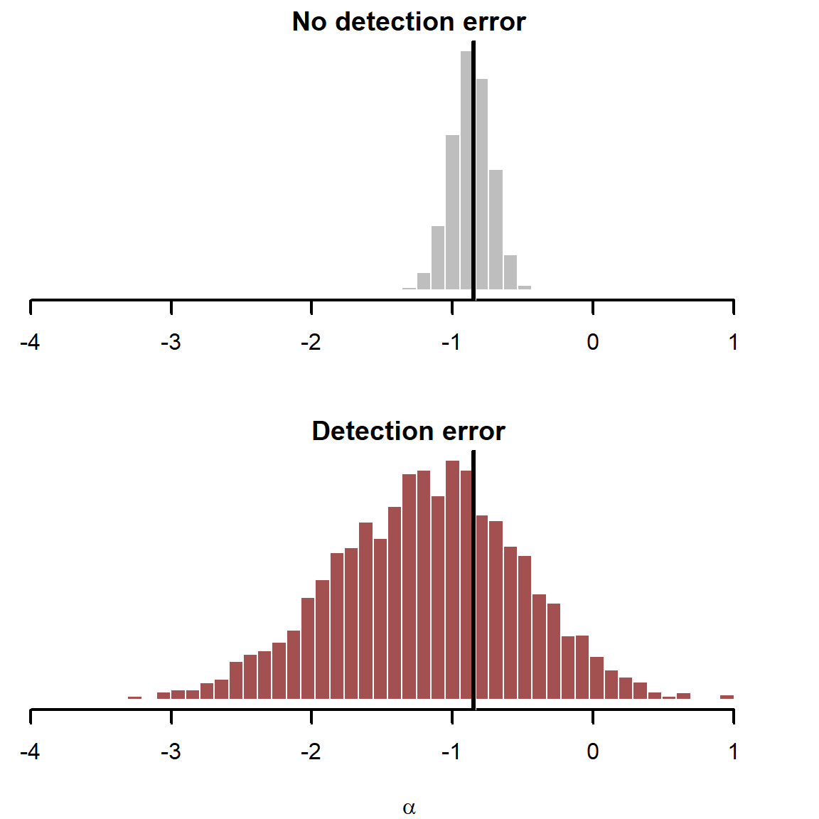
The detection error model seems to struggle estimating \(\alpha\) with precision, though our estimates are centred around the true simulated value. This parameter is a bit difficult to interpret in detection error models, so we will get back to that later. But our inferences on the effects of covariates are what we are primarily interested in. Next plot the estimated \(\beta\) coefficients for the two predictors, and again overlay the true simulated values in black
betas_noerror <- fit_noerror$draws("beta", format = "draws_matrix")
betas_error <- fit_error$draws("beta", format = "draws_matrix")
layout(matrix(1:4, ncol = 2, byrow = FALSE))
hist(betas_noerror[,1],
     col = 'grey', border = 'white', lwd = 2,
     xlim = range(c(betas_noerror[,1], betas_error[,1])),
     breaks = seq(min(c(betas_noerror[,1], betas_error[,1])),
                  max(c(betas_noerror[,1], betas_error[,1])),
                  length.out = 50),
     main = 'No detection error',
     yaxt = 'n', ylab = '', xlab = '')
abline(v = dat$true_betas[1], lwd = 3.5, col = 'white')
abline(v = dat$true_betas[1], lwd = 3, col = 'black')
hist(betas_error[,1],
     col = c_mid_highlight, border = 'white', lwd = 2,
     xlim = range(c(betas_noerror[,1], betas_error[,1])),
     breaks = seq(min(c(betas_noerror[,1], betas_error[,1])),
                  max(c(betas_noerror[,1], betas_error[,1])),
                  length.out = 50),
     main = 'Detection error', yaxt = 'n', ylab = '', xlab = expression(beta[1]))
abline(v = dat$true_betas[1], lwd = 3.5, col = 'white')
abline(v = dat$true_betas[1], lwd = 3, col = 'black')

hist(betas_noerror[,2],
     col = 'grey', border = 'white', lwd = 2,
     xlim = range(c(betas_noerror[,2], betas_error[,2])),
     main = 'No detection error',
     breaks = seq(min(c(betas_noerror[,2], betas_error[,2])),
                  max(c(betas_noerror[,2], betas_error[,2])),
                  length.out = 50),
     yaxt = 'n', ylab = '', xlab = '')
abline(v = dat$true_betas[2], lwd = 3.5, col = 'white')
abline(v = dat$true_betas[2], lwd = 3, col = 'black')
hist(betas_error[,2],
     col = c_mid_highlight, border = 'white', lwd = 2,
     xlim = range(c(betas_noerror[,2], betas_error[,2])),
     breaks = seq(min(c(betas_noerror[,2], betas_error[,2])),
                  max(c(betas_noerror[,2], betas_error[,2])),
                  length.out = 50),
     main = 'Detection error', yaxt = 'n', ylab = '', xlab = expression(beta[2]))
abline(v = dat$true_betas[2], lwd = 3.5, col = 'white')
abline(v = dat$true_betas[2], lwd = 3, col = 'black')
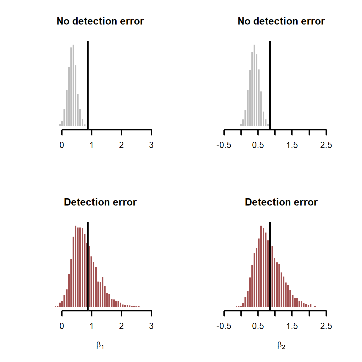
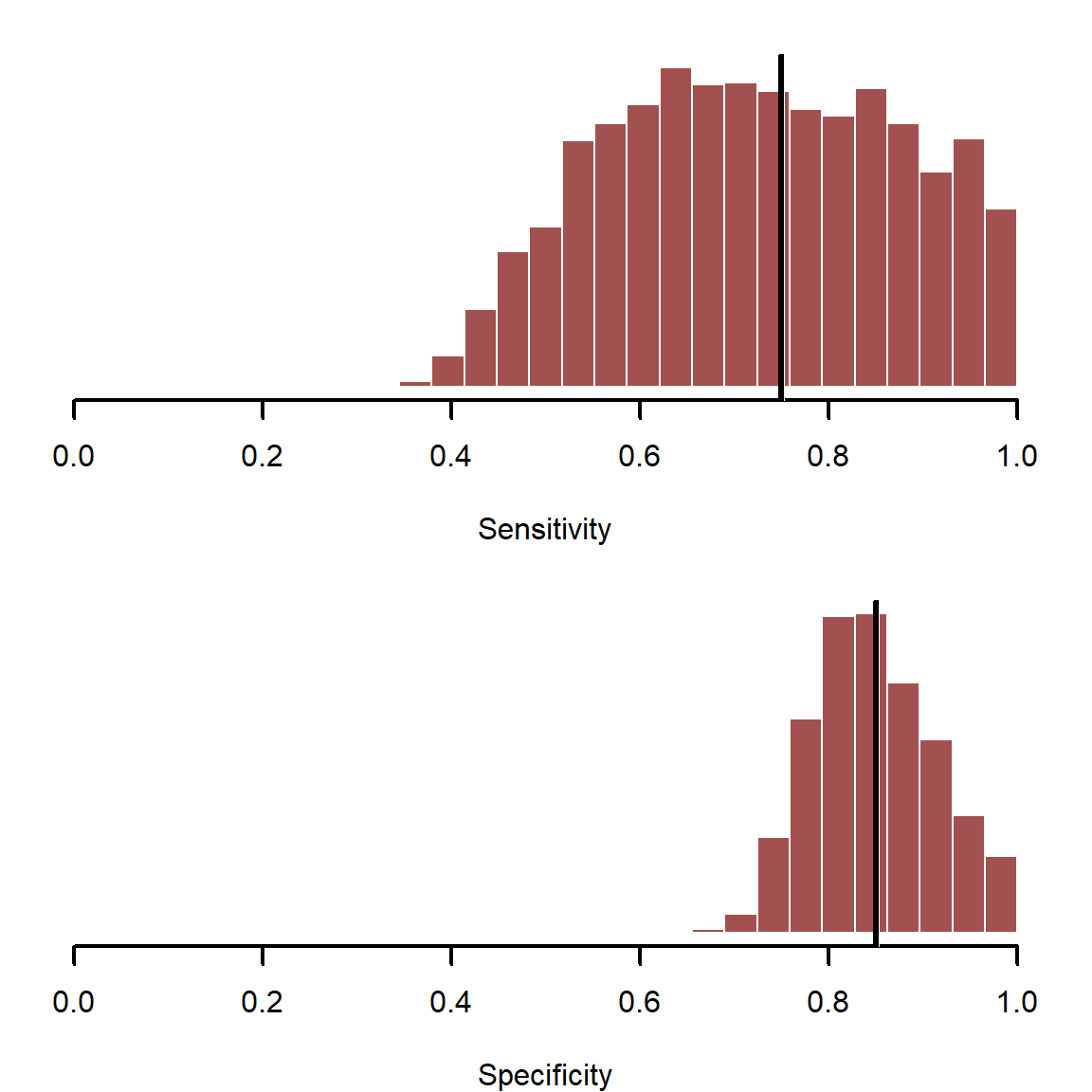
Here it is immediately clear why we should account for imperfect detection when possible. The detection error model gives better estimates for both coefficients. If we had to make decisions based on these parameters, and we did not account for detection error, our decisions would be wrong. Why is there large uncertainty in these estimates? To answer this, we need to plot the estimates for the test diagnostics
layout(matrix(1:2, ncol = 1))
par(mar = c(4, 1, 1.5, 1))
posterior_sens <- fit_error$draws("sens", format = "draws_matrix")
hist(posterior_sens,
     xlim = c(0, 1),
     breaks = seq(0, 1, length.out = 30),
     col = c_mid_highlight, border = 'white', lwd = 2,
     main = '', yaxt = 'n', ylab = '', xlab = 'Sensitivity')
abline(v = dat$true_sens, lwd = 3.5, col = 'white')
abline(v = dat$true_sens, lwd = 3, col = 'black')

posterior_spec <- fit_error$draws("spec", format = "draws_matrix")
hist(posterior_spec,
     xlim = c(0, 1),
     breaks = seq(0, 1, length.out = 30),
     col = c_mid_highlight, border = 'white', lwd = 2,
     main = '', yaxt = 'n', ylab = '', xlab = 'Specificity')
abline(v = dat$true_spec, lwd = 3.5, col = 'white')
abline(v = dat$true_spec, lwd = 3, col = 'black')
Further investigation helps to diagnose why \(\alpha\) is difficult to identify for the detection error model.
layout(matrix(1:2, ncol = 1))
par(mar = c(4, 4, 1.5, 1))
posterior_sens <- fit_error$draws("sens", format = "draws_matrix")
plot(alphas_error, posterior_sens,  xlab = '',
     ylab = 'Sensitivity', bty = 'l', pch = 16, col = c_mid_highlight)
box(bty = 'l', lwd = 2)
abline(h = dat$true_sens, lwd = 3.5, col = 'white')
abline(h = dat$true_sens, lwd = 3, col = 'black')
abline(v = dat$true_alpha, lwd = 3.5, col = 'white')
abline(v = dat$true_alpha, lwd = 3, col = 'black')

posterior_spec <- fit_error$draws("spec", format = "draws_matrix")
plot(alphas_error, posterior_spec,  xlab = expression(alpha),
     ylab = 'Specificity', bty = 'l', pch = 16, col = c_mid_highlight)
box(bty = 'l', lwd = 2)
abline(h = dat$true_spec, lwd = 3.5, col = 'white')
abline(h = dat$true_spec, lwd = 3, col = 'black')
abline(v = dat$true_alpha, lwd = 3.5, col = 'white')
abline(v = dat$true_alpha, lwd = 3, col = 'black')
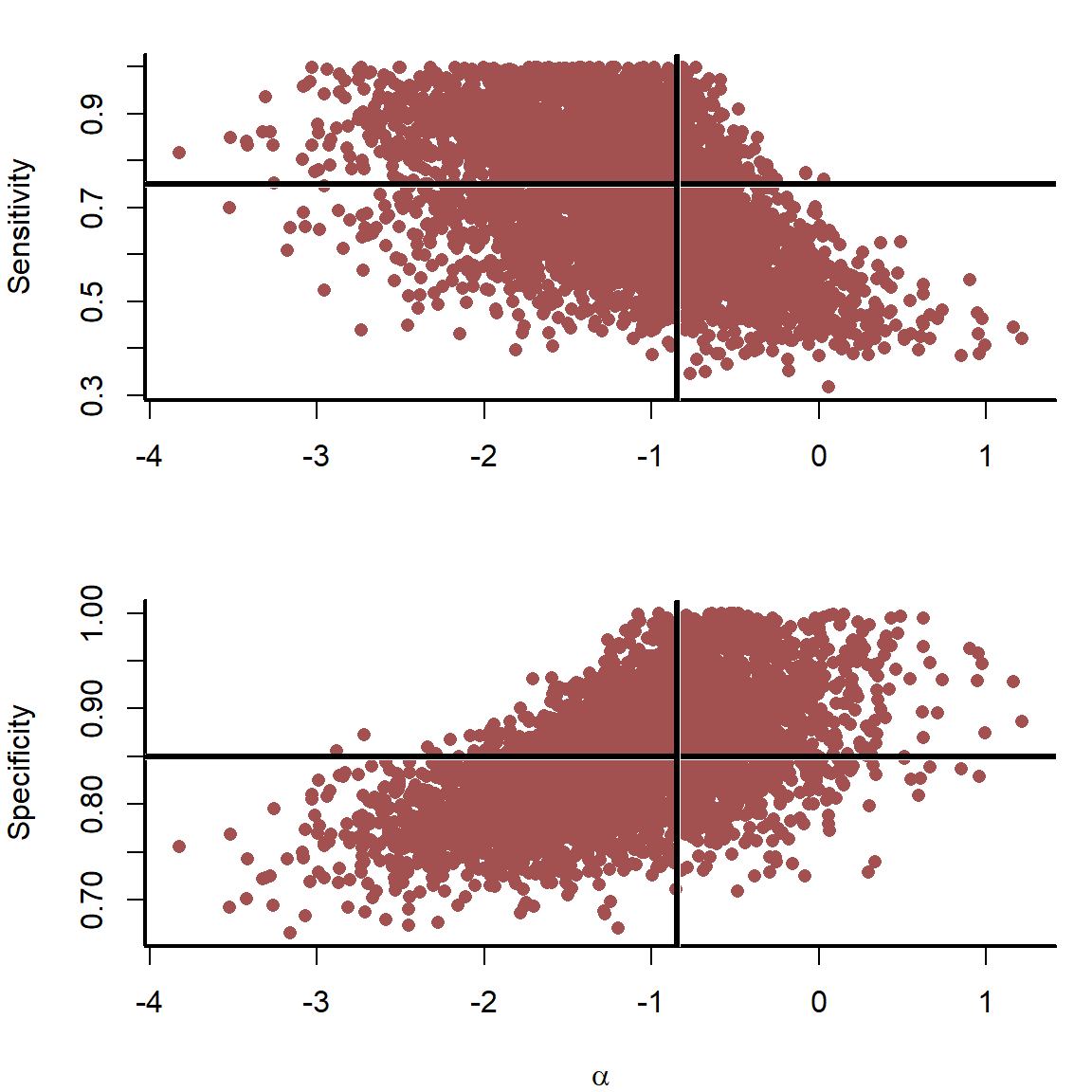
There are fundamental posterior correlations induced between \(\alpha\) and sensitivity and between \(\alpha\) and specificity. This model cannot estimate sensitivity or specificity with much precision, resulting in wide estimates of \(\alpha\). There is nothing implicitly wrong here, these uncertainties simply reflect reality: We do not know the true infection status, and we do not know the true test performance. Without knowing these, how can we precisely estimate the average infection probability \(\alpha\)? Stronger priors on diagnostic accuracies could help, but these uncertainties will not entirely go away without sampling many more individuals.
A very useful question raised by
A/Prof Joerg Henning relates to translating what these results might mean for a practicing clinician. Often we want to know how likely it is that a person is truly infected if they’ve returned a positive diagnostic test. A famous (and very topical) problem in probability theory is the
base rate fallacy. This occurs when we ignore the background rate (or prevalence of disease, in our case) when interpreting test results. No test is perfect, so they will sometimes return false positives. But if there are very few true positives in the population (because the disease is rare), this can mean that a high proportion of people testing positive are actually uninfected. To quote from
Wikipedia: “It is especially counter-intuitive when interpreting a positive result in a test on a low-prevalence population after having dealt with positive results drawn from a high-prevalence population. If the false positive rate of the test is higher than the proportion of the new population with the condition, then a test administrator whose experience has been drawn from testing in a high-prevalence population may conclude from experience that a positive test result usually indicates a positive subject, when in fact a false positive is far more likely to have occurred.”
We can use sampling from our model’s joint posterior distribution to calculate the probability that someone returning a positive test is actually infected, which requires the following equation:
$$Pr(true~infect|pos~test) = Pr(pos~test|true~infect) * Pr(infected) /
 (Pr(pos~test|true~infect) * Pr(infect) + Pr(pos~test|true~uninfect) * Pr(uninfect))$$
For details of this derivation, please read here and here).
Because I’m no wizard in probability theory, I’ll use brute force sampling to calculate this quantity. First, create a sample sequence to generate many posterior simulations. We do this because we want many thousands of samples, but we only have 4000 in our posterior.
N_samples <- 25000
sample_seq <- sample(1:NROW(posterior_sens), N_samples, replace = TRUE)
Next, sample latent (true) infection status for 25000 individuals using the logistic regression equation estimated by our model
true_inf <- matrix(NA, nrow = N_samples, ncol = NROW(dat$x))
for(i in 1:N_samples){
  true_inf[i,] <- rbinom(NROW(dat$x),
                         size = 1,
                         prob = boot::inv.logit(alphas_error[sample_seq[i]] +
                                                  dat$x %*% as.vector(betas_noerror[sample_seq[i],])))
}
Sample observed test diagnostics given our model’s estimates for sensitivity and specificity
test_results <- matrix(NA, nrow = N_samples, ncol = NROW(dat$x))
for(i in 1:N_samples){
  for(j in 1:NCOL(test_results)){
    test_results[i,j] <- ifelse(true_inf[i,j] == 1,
                                rbinom(n = 1,
                                       size = 1,
                                       prob = posterior_sens[sample_seq[i]]),
                                rbinom(n = 1,
                                       size = 1,
                                       prob = 1 - posterior_spec[sample_seq[i]]))
  }
}
Now we have all the samples we need to calculate relevant probabilistic quantities. Calculate the probability that an individual returns a positive test if they are actually infected. We would hope this value would be high, but that is not always the case
`Pr(positive test|truly infected)` <- vector(length = N_samples)
for(i in 1:N_samples){
  `Pr(positive test|truly infected)`[i] = sum(test_results[i, which(true_inf[i,] == 1)]) /
    length(which(true_inf[i,] == 1))
}
quantile(`Pr(positive test|truly infected)`, probs = c(0.1, 0.25, 0.5, 0.75, 0.9))
##       10%       25%       50%       75%       90%
## 0.5000000 0.5967742 0.7241379 0.8529412 0.9428571
Next calculate the probability that any individual in the population is infected (prevalence)
`Pr(infected)` <- vector(length = N_samples)
for(i in 1:N_samples){
  `Pr(infected)`[i] = sum(true_inf[i,]) / length(true_inf[i,])
}
quantile(`Pr(infected)`, probs = c(0.1, 0.25, 0.5, 0.75, 0.9))
##   10%   25%   50%   75%   90%
## 0.124 0.180 0.256 0.348 0.440
Now we need the probability of returning a positive test if someone is truly uninfected. We would hope this value would be quite low
`Pr(positive test|truly uninfected)` <- vector(length = N_samples)
for(i in 1:N_samples){
  `Pr(positive test|truly uninfected)`[i] = sum(test_results[i, which(true_inf[i,] == 0)]) /
    length(which(true_inf[i,] == 0))
}
quantile(`Pr(positive test|truly uninfected)`, probs = c(0.1, 0.25, 0.5, 0.75, 0.9))
##        10%        25%        50%        75%        90%
## 0.05552764 0.10256410 0.15384615 0.20105820 0.24117647
Now the probability that any individual is uninfected, which is 1 - Pr(infected)
`Pr(uninfected)` <- vector(length = N_samples)
for(i in 1:N_samples){
  `Pr(uninfected)`[i] = 1 - `Pr(infected)`[i]
}
quantile(`Pr(uninfected)`, probs = c(0.1, 0.25, 0.5, 0.75, 0.9))
##   10%   25%   50%   75%   90%
## 0.560 0.652 0.744 0.820 0.876
Finally, we can calculate our quantity of interest: the probability that an individual is actually infected if they return a positive test
`Pr(truly infected|positive test)` <- vector(length = N_samples)
for(i in 1:N_samples){
  `Pr(truly infected|positive test)`[i] = `Pr(positive test|truly infected)`[i] * `Pr(infected)`[i] /
    (`Pr(positive test|truly infected)`[i] * `Pr(infected)`[i] +
       `Pr(positive test|truly uninfected)`[i] * `Pr(uninfected)`[i])
}
hist(`Pr(truly infected|positive test)`,
     xlim = c(0, 1),
     breaks = seq(0, 1, length.out = 30),
     col = c_mid_highlight, border = 'white', lwd = 2,
     main = '', yaxt = 'n', ylab = '',
     xlab = 'Pr(truly infected|positive test)')
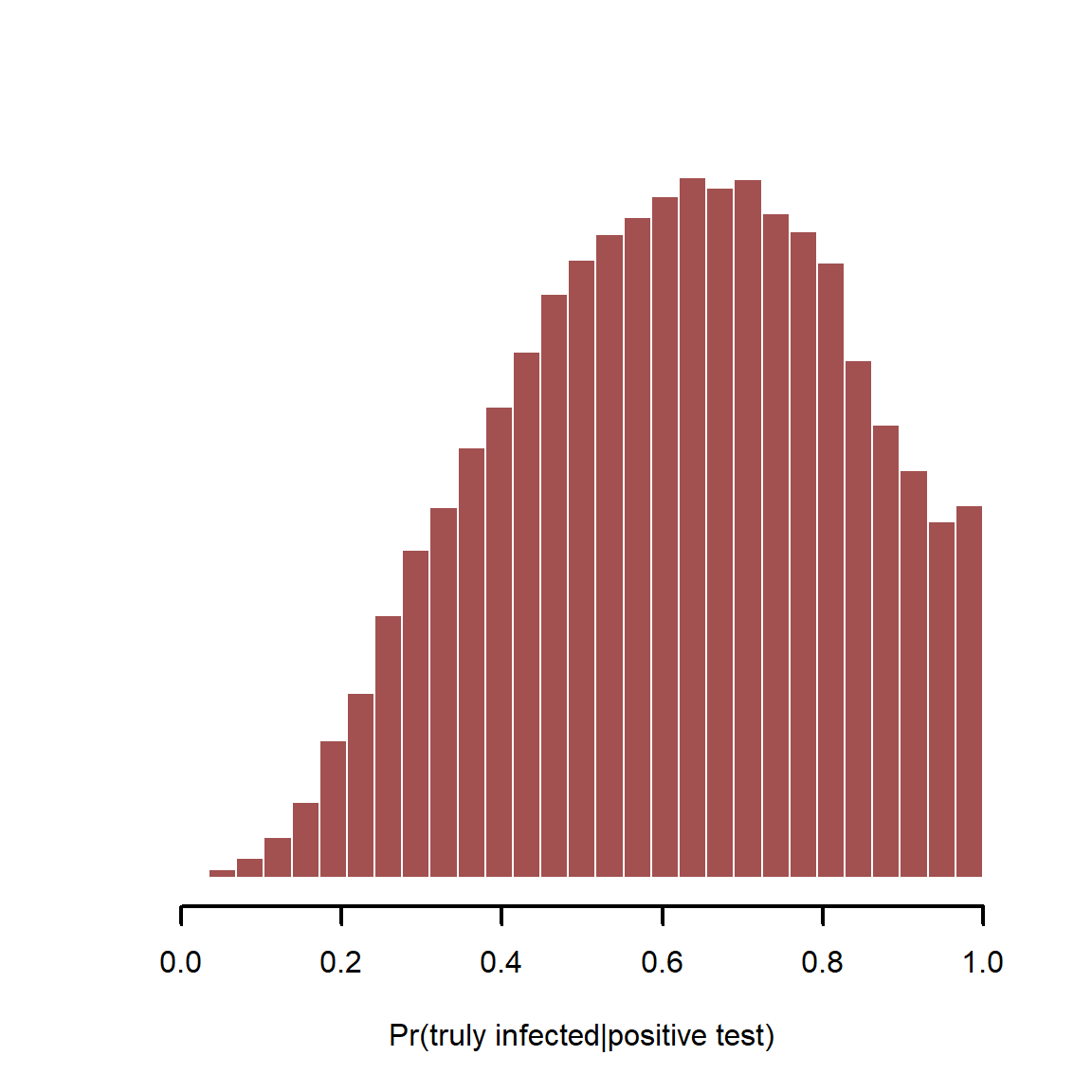
With imperfect tests and somewhat rare infections (~30% in this example), we can’t be too sure that a positive test means a true infection. This all changes of course if we have other reasons to believe a person is infected. For example, if we only test people that show some symptoms, we are sampling a very different population compared to the full population of healthy and unhealthy individuals. Hopefully this example illustrates why simple logistic regressions are often not enough to tackle the questions we are interested in.