Simulating data for model exploration in R
By Nicholas Clark in rstats simulation
March 12, 2024
Purpose
The following passage is quoted directly from Regression and other stories (Gelman, Hill and Vehtari 2022). “Simulation of random variables is important in applied statistics for several reasons. First, we use probability models to mimic variation in the world, and the tools of simulation can help us better understand how this variation plays out. Patterns of randomness are notoriously contrary to normal human thinking—our brains don’t seem to be able to do a good job understanding that random swings will be present in the short term but average out in the long run—and in many cases simulation is a big help in training our intuitions about averages and variation. Second, we can use simulation to approximate the sampling distribution of data and propagate this to the sampling distribution of statistical estimates and procedures. Third, regression models are not deterministic; they produce probabilistic predictions. Simulation is the most convenient and general way to represent uncertainties in forecasts”
This script walks through some potential uses of simulation, but it is by no means exhaustive. First, generate some nice plotting colours
c_light <- c("#DCBCBC")
c_light_highlight <- c("#C79999")
c_mid <- c("#B97C7C")
c_mid_highlight <- c("#A25050")
c_dark <- c("#8F2727")
c_dark_highlight <- c("#7C0000")
Next we define a few helper functions for making nice plots
myhist = function(x,
                  xlim,
                  xlab = '',
                  main = ''){
  if(missing(xlim)){
    xlim <- range(x)
  }

  hist(x,
       xlim = xlim,
       yaxt = 'n',
       xlab = xlab,
       ylab = '',
       col = c_mid_highlight,
       border = 'white',
       lwd = 2,
       breaks = 20,
       main = main)
}

myscatter = function(x,
                     y,
                     xlab = '',
                     ylab = ''){
  plot(x = x,
       y = y,
       pch = 16,
       col = 'white',
       cex = 1.25,
       bty = 'l',
       xlab = xlab,
       ylab = ylab)
  points(x = x, y = y, pch = 16,
         col = c_dark,
         cex = 1)
  box(bty = 'l', lwd = 2)
}

mypred_plot = function(predictions, pred_values,
                       ylim,
                       ylab = 'Predictions', xlab = 'Covariate'){
  probs <- c(0.05, 0.2, 0.3, 0.4, 0.5, 0.6, 0.7, 0.8, 0.95)
  cred <- sapply(1:NROW(predictions),
                 function(n) quantile(predictions[n,],
                                      probs = probs, na.rm = TRUE))

  if(missing(ylim)){
    ylim <- range(cred)
  }

  plot(1, type = "n", bty = 'L',
       xlab = xlab,
       ylab = ylab,
       xlim = range(pred_values),
       ylim = ylim)

  polygon(c(pred_values, rev(pred_values)), c(cred[1,], rev(cred[9,])),
          col = c_light, border = NA)
  polygon(c(pred_values, rev(pred_values)), c(cred[2,], rev(cred[8,])),
          col = c_light_highlight, border = NA)
  polygon(c(pred_values, rev(pred_values)), c(cred[3,], rev(cred[7,])),
          col = c_mid, border = NA)
  polygon(c(pred_values, rev(pred_values)), c(cred[4,], rev(cred[6,])),
          col = c_mid_highlight, border = NA)
  lines(pred_values, cred[5,], col = c_dark, lwd = 2.5)

  box(bty = 'l', lwd = 2)
}
Simulating a simple linear regression
A linear regression generally assumes additive, linear effects of predictors on the mean of a response variable. It also assumes the errors (unexplained variation) are independent and identically distributed (i.e. the same variance / sd) applies to the full distribution of errors. We will simulate a vegetation cover outcome variable under the following model:
$$\boldsymbol{vegetation}\sim \text{Normal}(\mu,\sigma)$$
A linear predictor is modeled on the \(identity\) scale to capture effects of covariates on \(\mu\):
$$\mu=\alpha+{\beta_{temp}}*\boldsymbol{temperature}$$
We simulate data with a single predictor, \(temperature\), and with varying sample sizes to inspect the influence of sample size on our inferences. Start with a sample size of 300.
N <- 300
First we will simulate the predictor variable, \(temperature\). Our first decision is to think about what distribution the predictor might have. For many modelling approaches, it is often useful to transform continuous predictors so they are standard normal in distribution (i.e. \(\boldsymbol{temperature}\sim \text{Normal}(0,1)\)). This might be the case if we were to measure temperature and then standardise it to unit variance
set.seed(1971)
temperature_raw <- rnorm(n = N, mean = 14, sd = 5)
myhist(temperature_raw, xlab = 'Raw temperature')
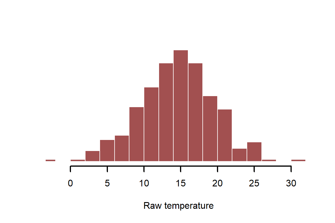
It is often useful to standardize variables to unit variance before modelling; this helps us to compare effects from different predictors but also helps to specify useful prior distributions when fitting Bayesian models. This is most commonly done by shifting the mean to 0 and dividing by 1sd
temperature_scaled <- (temperature_raw - mean(temperature_raw)) /
  sd(temperature_raw)
myhist(temperature_scaled, xlab = 'Scaled temperature')
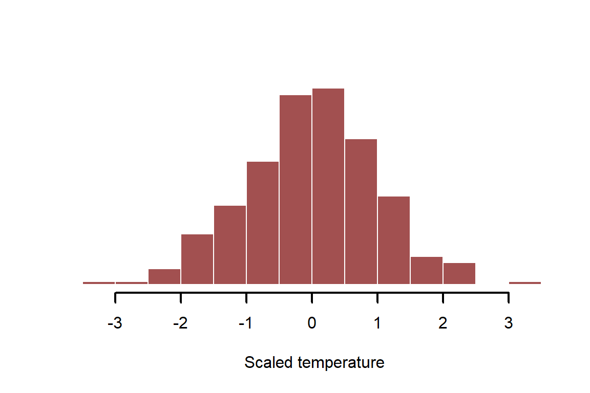
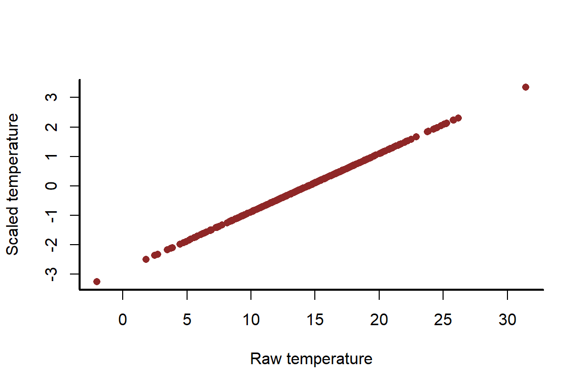
This shifts the distribution but it does not change the properties of the variable
myscatter(x = temperature_raw,
          y = temperature_scaled,
          xlab = 'Raw temperature',
          ylab = 'Scaled temperature')
Now simulate the actual linear effect of \(temperature\) on the mean of our outcome, \(vegetation\). This is captured by the coefficient \({\beta_{temp}}\)
beta_temp <- 0.25
Next we need to simulate the intercept \(\alpha\). This parameter represents the average vegetation when temperature is at 0
alpha <- 1
The other parameter we need to simulate is the standard deviation of the errors \(\sigma\); we don’t expect that temperature is the only mechanism influencing vegetation, so we need to include unexplained variation
sigma <- 2
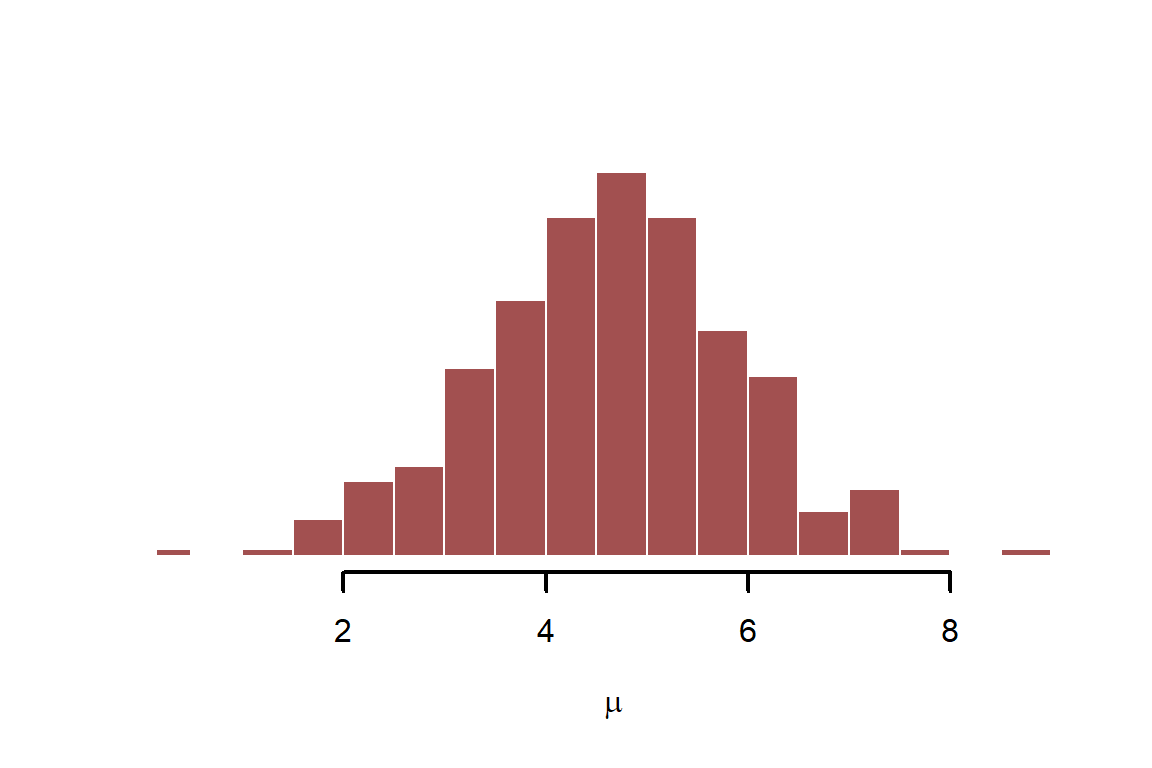
Finally, we have the components to simulate our outcome variable, \(vegetation\). Simulate the linear predictor, which is \(\mu=\alpha+{\beta_{temp}}*\boldsymbol{temperature}\)
mu <- alpha + beta_temp * temperature_raw
myhist(mu, xlab = expression(mu))
Next, complete the probabilistic data generation by simulating the observations. Here we assume vegetation is normally distributed, so we use the random number generator rnorm(). Use ?rnorm to learn more about normal distribution functions in R
vegetation <- rnorm(n = N, mean = mu, sd = sigma)
myhist(vegetation, xlab = 'Vegetation')
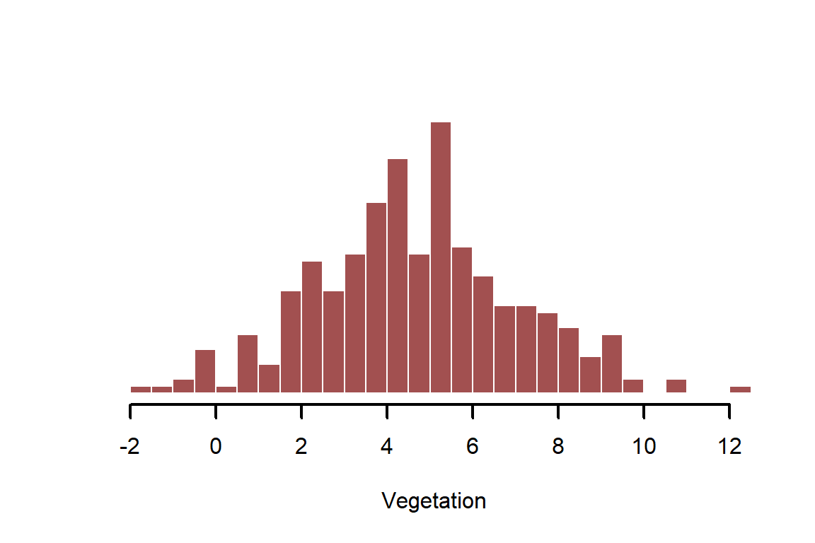
There should be an obvious positive relationship between raw \(temperature\) and \(vegetation\); but it also shouldn’t be a perfect 1:1 relationship
myscatter(x = temperature_raw,
          y = vegetation,
          xlab = 'Raw temperature',
          ylab = 'Vegetation')
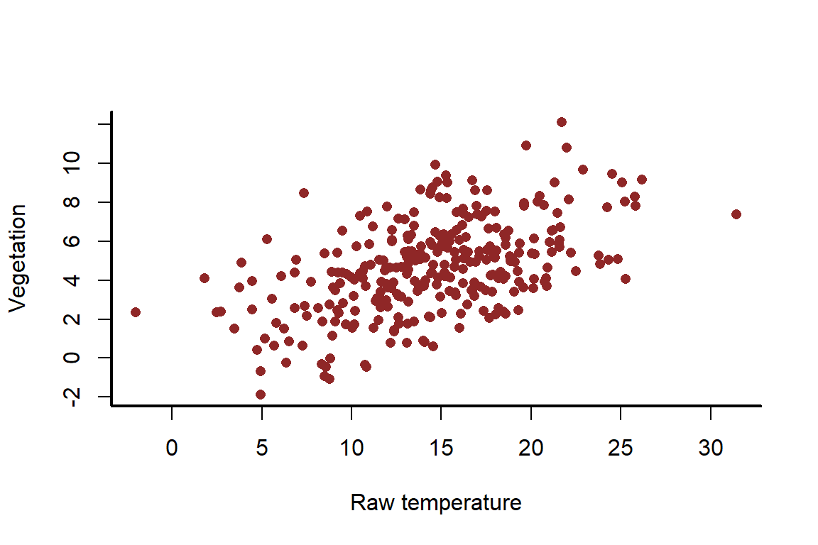
We can now estimate the effect of temperature on the mean of vegetation using the lm() function in R. This function uses iteratively reweighted least squares to estimate model parameters in a maximum likelihood framework. But we will use the scaled version of temperature to showcase how this gives us coefficients that we can still interpret
veg_mod <- lm(vegetation ~ temperature_scaled)
summary(veg_mod)
##
## Call:
## lm(formula = vegetation ~ temperature_scaled)
##
## Residuals:
##     Min      1Q  Median      3Q     Max
## -4.3773 -1.4182 -0.0611  1.2073  5.6760
##
## Coefficients:
##                    Estimate Std. Error t value Pr(>|t|)
## (Intercept)          4.6737     0.1168   40.01   <2e-16 ***
## temperature_scaled   1.2222     0.1170   10.45   <2e-16 ***
## ---
## Signif. codes:  0 '***' 0.001 '**' 0.01 '*' 0.05 '.' 0.1 ' ' 1
##
## Residual standard error: 2.023 on 298 degrees of freedom
## Multiple R-squared:  0.268,	Adjusted R-squared:  0.2655
## F-statistic: 109.1 on 1 and 298 DF,  p-value: < 2.2e-16
The coefficients are harder to interpret now because we scaled the predictor
coef(veg_mod)
##        (Intercept) temperature_scaled
##           4.673721           1.222223
Compare these estimates to the true values
cbind(alpha, beta_temp)[1,]
##     alpha beta_temp
##      1.00      0.25
Both of these coefficients need to be interpreted by taking into account the standard deviation of the predictor variable, \(vegetation\). Once we back-transform, we can see the point estimates are very close to the true simulated values. This is a useful first check to ensure the model is able to recover simulated parameters. It is always surprising how often a model is not able to recover these when we simulate, especially for more complex models / simulations
coef(veg_mod) / sd(temperature_raw)
##        (Intercept) temperature_scaled
##          0.9237536          0.2415704
We can also calculate uncertainties of these coefficients, again on the appropriate scale
confint(veg_mod) / sd(temperature_raw)
##                        2.5 %    97.5 %
## (Intercept)        0.8783128 0.9691943
## temperature_scaled 0.1960538 0.2870871
Finally, for most maximum likelihood models in R (lm, glm, gam etc….) we can draw samples of regression coefficients from the implied posterior distribution. Maximum likelihood finds the posterior mode and then uses gradients around the mode to approximate the posterior with a Gaussian (Normal) distribution. So the posterior of coefficients is always multivariate normal. All we need to generate samples from this posterior is the variance-covariance matrix and the mean coefficients
mean_coefs <- coef(veg_mod)
coef_vcv <- vcov(veg_mod)
Generate 2,000 regression coefficient samples from the implied multivariate normal posterior distribution. We can use the mvrnorm() function from the MASS package to make this simple
if(!require(MASS)){
  install.packages('MASS')
}
## Loading required package: MASS
coef_posterior <- MASS::mvrnorm(n = 2000,
                                mu = mean_coefs,
                                Sigma = coef_vcv)
head(coef_posterior)
##      (Intercept) temperature_scaled
## [1,]    4.821914          1.2911135
## [2,]    4.572132          1.2185941
## [3,]    4.612218          1.4297919
## [4,]    4.534363          1.3223695
## [5,]    4.636644          1.3577525
## [6,]    4.866013          0.9418046
Instead of simply looking at confidence intervals of coefficients, we can now inspect the full distribution and overlay the true simulated value. Remember to adjust for the scaling of the variable
myhist(x = coef_posterior[,2] / sd(temperature_raw),
       xlab = 'Posterior temp coefficient (unscaled)')
abline(v = beta_temp, lwd = 3, col = 'white')
abline(v = beta_temp, lwd = 2.5, col = 'black')
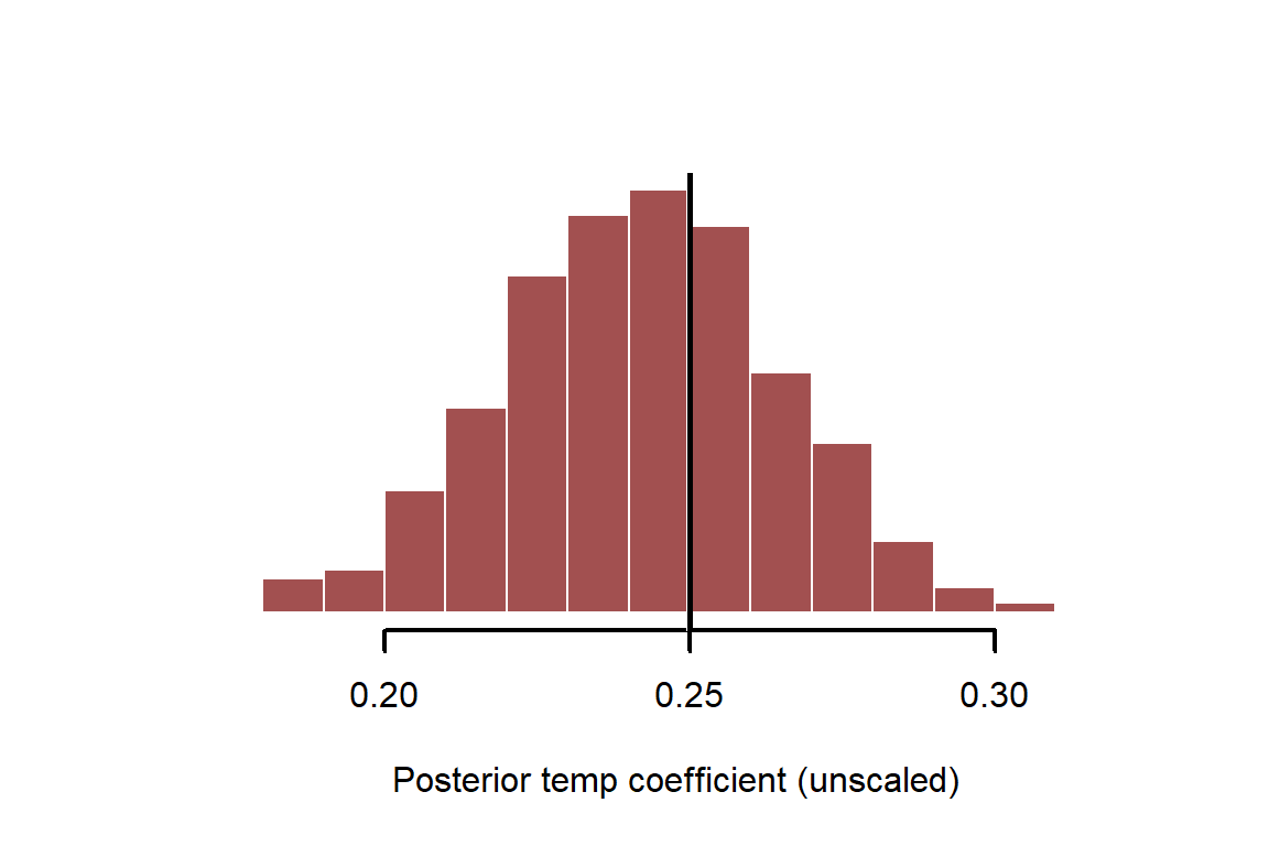
Prediction intervals can also be obtained once we have the posterior estimates. Predicting from models is a crucial step to understand them and interrogate their weaknesses. To make predictions, we usually must supply newdata for predicting against. This would mean a new set of temperature measurements, in our case. The best way to do this, depending on model complexity, is to create a sequence of measurements for the variable of interest that we’d like predictions for. See ?predict.lm for more details
newtemps <- seq(from = min(temperature_scaled),
                to = max(temperature_scaled),
                length.out = 1000)
summary(newtemps)
##     Min.  1st Qu.   Median     Mean  3rd Qu.     Max.
## -3.26551 -1.61228  0.04094  0.04094  1.69416  3.34738
Create an empty matrix to store the predictions. We want to predict at these new \(temperature\) values for each combination of posterior coefficients so we can visualise uncertainty in those predictions
predictions <- matrix(NA, ncol = NROW(coef_posterior),
                      nrow = length(newtemps))
dim(predictions)
## [1] 1000 2000
Now fill the matrix with the predicted mean for each of the new \(temperature\) measurements, using each posterior draw of regression coefficients
for(i in 1:NCOL(predictions)){
  predictions[,i] <- coef_posterior[i,1] + (coef_posterior[i,2] * newtemps)
}
Plot empirical quantile ribbons of the predictions to visualise them, and overlay the simulated values as points
mypred_plot(predictions = predictions,
            xlab = 'Temperature (scaled)',
            ylab = 'Vegetation (expectation only)',
            pred_values = newtemps,
            ylim = range(c(vegetation,
                           quantile(predictions, probs = c(0.025, 0.975)))))
points(pch = 16, x = temperature_scaled, y = vegetation,
       col = 'white',
       cex = 1)
points(pch = 16, x = temperature_scaled, y = vegetation,
       cex = 0.8)
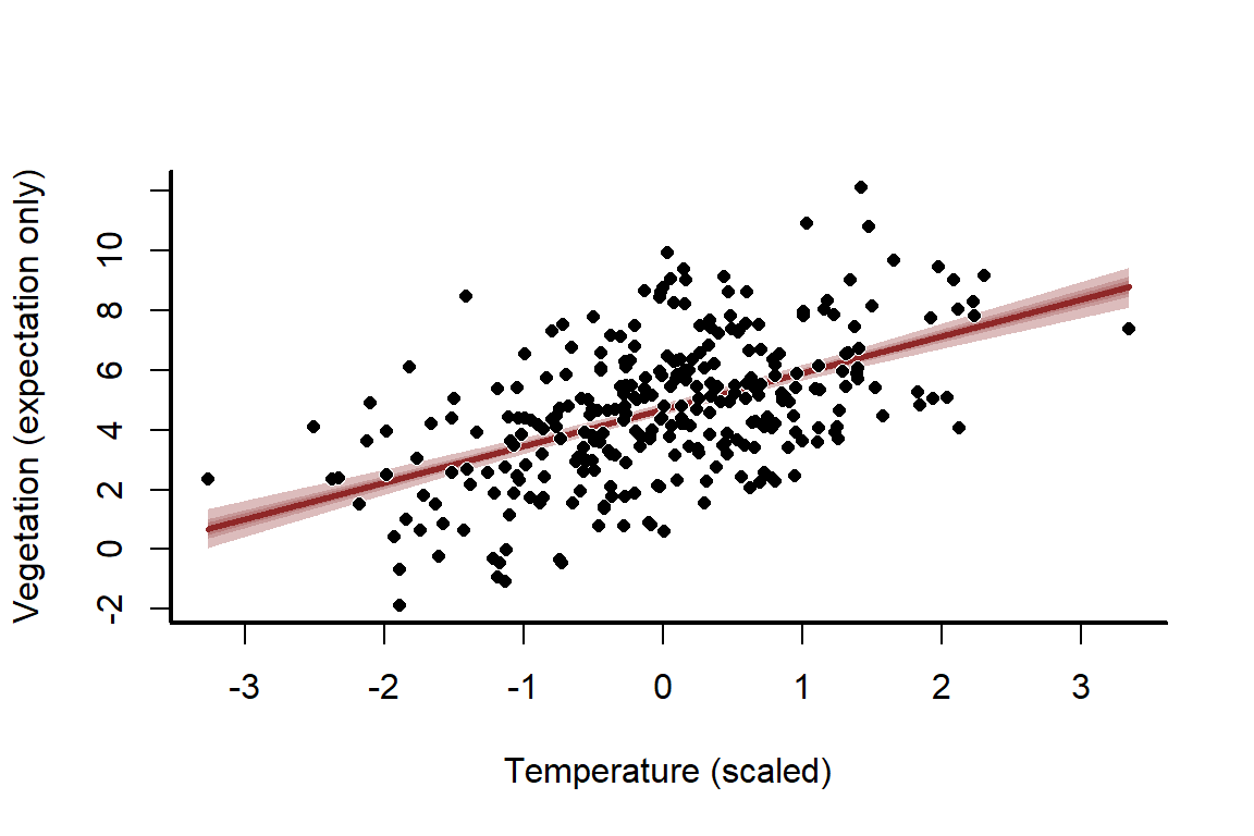
The uncertainty about this line seems far too narrow, and that’s because it is! We have ignored the stochastic component, which is the normally distributed errors. This means we have only predicted the mean, otherwise known as the expectation. But we can easily compute full probabilistic predictions and re-plot. All we need is the sd estimate for \(\sigma\), which is stored as sigma in the model. This estimate is extremely close to our true simulated value
sigma_estimate <- summary(veg_mod)$sigma
sigma_estimate; sigma
## [1] 2.023472
## [1] 2
Now compute predictions using normal random draws with appropriate probabilistic uncertainty
predictions <- matrix(NA, ncol = NROW(coef_posterior),
                      nrow = length(newtemps))
for(i in 1:NCOL(predictions)){
  predictions[,i] <- rnorm(n = NROW(predictions),
                           mean = coef_posterior[i,1] + (coef_posterior[i,2] * newtemps),
                           sd = sigma_estimate)
}
Plot the full prediction distribution
mypred_plot(predictions = predictions,
            xlab = 'Temperature (scaled)',
            ylab = 'Vegetation (full uncertainty)',
            pred_values = newtemps,
            ylim = range(c(vegetation,
                           quantile(predictions, probs = c(0.025, 0.975)))))
points(pch = 16, x = temperature_scaled, y = vegetation,
       col = 'white',
       cex = 1)
points(pch = 16, x = temperature_scaled, y = vegetation,
       cex = 0.8)
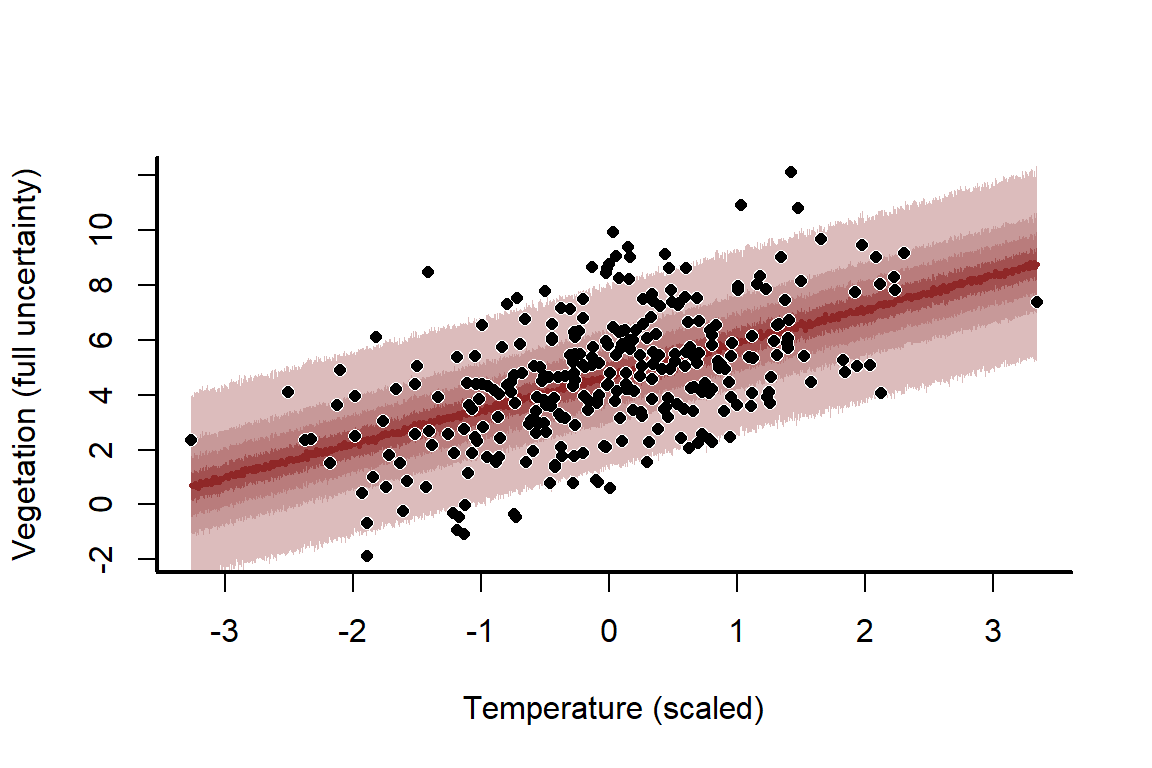
This model fits the data very well, with good coverage properties of the prediction uncertainties. But what happens if we decrease the sample size to 10 and run the process again?
N <- 10
temperature_raw <- rnorm(n = N, mean = 14, sd = 5)
temperature_scaled <- (temperature_raw - mean(temperature_raw)) /
  sd(temperature_raw)
mu <- alpha + beta_temp * temperature_raw
vegetation <- rnorm(n = N, mean = mu, sd = sigma)
veg_mod <- lm(vegetation ~ temperature_scaled)
mean_coefs <- coef(veg_mod); coef_vcv <- vcov(veg_mod)
coef_posterior_new <- MASS::mvrnorm(n = 2000,
                                mu = mean_coefs,
                                Sigma = coef_vcv)
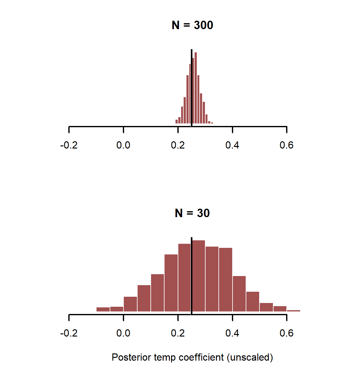
Plot posterior estimates from both simulations, but use the same x-axis limits so the distributions can be compared
layout(matrix(1:2, nrow = 2))
myhist(x = coef_posterior[,2] / sd(temperature_raw),
       xlim = range(c(coef_posterior[,2] / sd(temperature_raw),
                    coef_posterior_new[,2] / sd(temperature_raw))),
       xlab = '', main = 'N = 300')
abline(v = beta_temp, lwd = 3, col = 'white')
abline(v = beta_temp, lwd = 2.5, col = 'black')

myhist(x = coef_posterior_new[,2] / sd(temperature_raw),
       xlim = range(c(coef_posterior[,2] / sd(temperature_raw),
                      coef_posterior_new[,2] / sd(temperature_raw))),
       xlab = 'Posterior temp coefficient (unscaled)',
       main = 'N = 30')
abline(v = beta_temp, lwd = 3, col = 'white')
abline(v = beta_temp, lwd = 2.5, col = 'black')
layout(1)
How does this wider uncertainty translate into the predictions?
sigma_estimate <- summary(veg_mod)$sigma
predictions <- matrix(NA, ncol = NROW(coef_posterior_new),
                      nrow = length(newtemps))
for(i in 1:NCOL(predictions)){
  predictions[,i] <- rnorm(n = NROW(predictions),
                           mean = coef_posterior_new[i,1] + (coef_posterior_new[i,2] * newtemps),
                           sd = sigma_estimate)
}
mypred_plot(predictions = predictions,
            xlab = 'Temperature (scaled)',
            ylab = 'Vegetation (full uncertainty)',
            pred_values = newtemps,
            ylim = range(c(vegetation,
                           quantile(predictions, probs = c(0.025, 0.975)))))
points(pch = 16, x = temperature_scaled, y = vegetation,
       col = 'white',
       cex = 1)
points(pch = 16, x = temperature_scaled, y = vegetation,
       cex = 0.8)
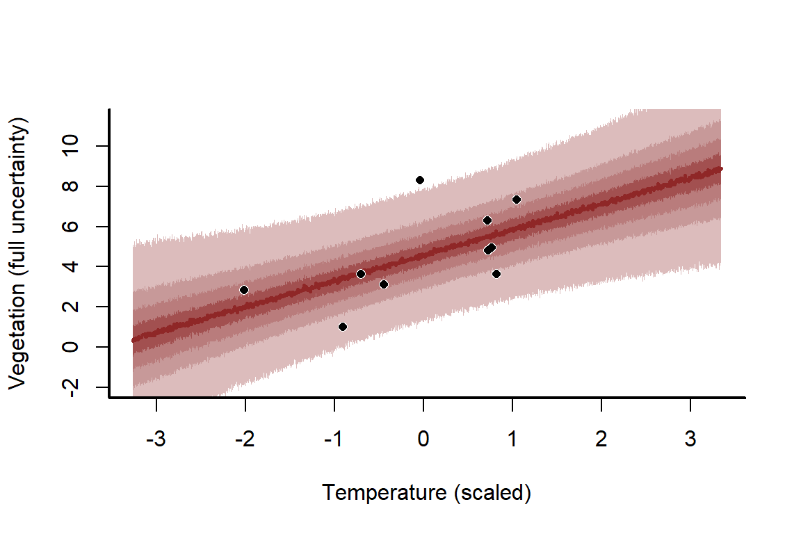
Changing sample size is just one way to get a feel for how challenging some modelling problems can be to tackle. You can also change \(\sigma\), the \({\beta_{temp}}\) coefficient, and / or the \(\alpha\) coefficient to understand what those changes might mean
Inspecting confounding and its influence on causal inferences
In this next example, we will simulate a data-generating process that has a strong confounder (in the form of a collider). This will illustrate how wrong our conclusions can be if we simply throw all variables into a regression and interpret them as real risk factors / causal effects. We will use a similar approach as above, where the goal is to model \(vegetation\) density
set.seed(11155)
N <- 100
\(temperature\) again is our main predictor of interest. This time we’ll ignore the scaling and just run with the scaled version for simplicity
temperature <- rnorm(N,
                     mean = 0,
                     sd = 1)
\(temperature\) again has a strong positive, linear effect on \(vegetation\)
beta_temp <- 0.75
vegetation <- rnorm(N,
                    mean = beta_temp * temperature,
                    sd = 1)
myscatter(x = temperature,
          y = vegetation,
          xlab = 'Temperature',
          ylab = 'Vegetation')
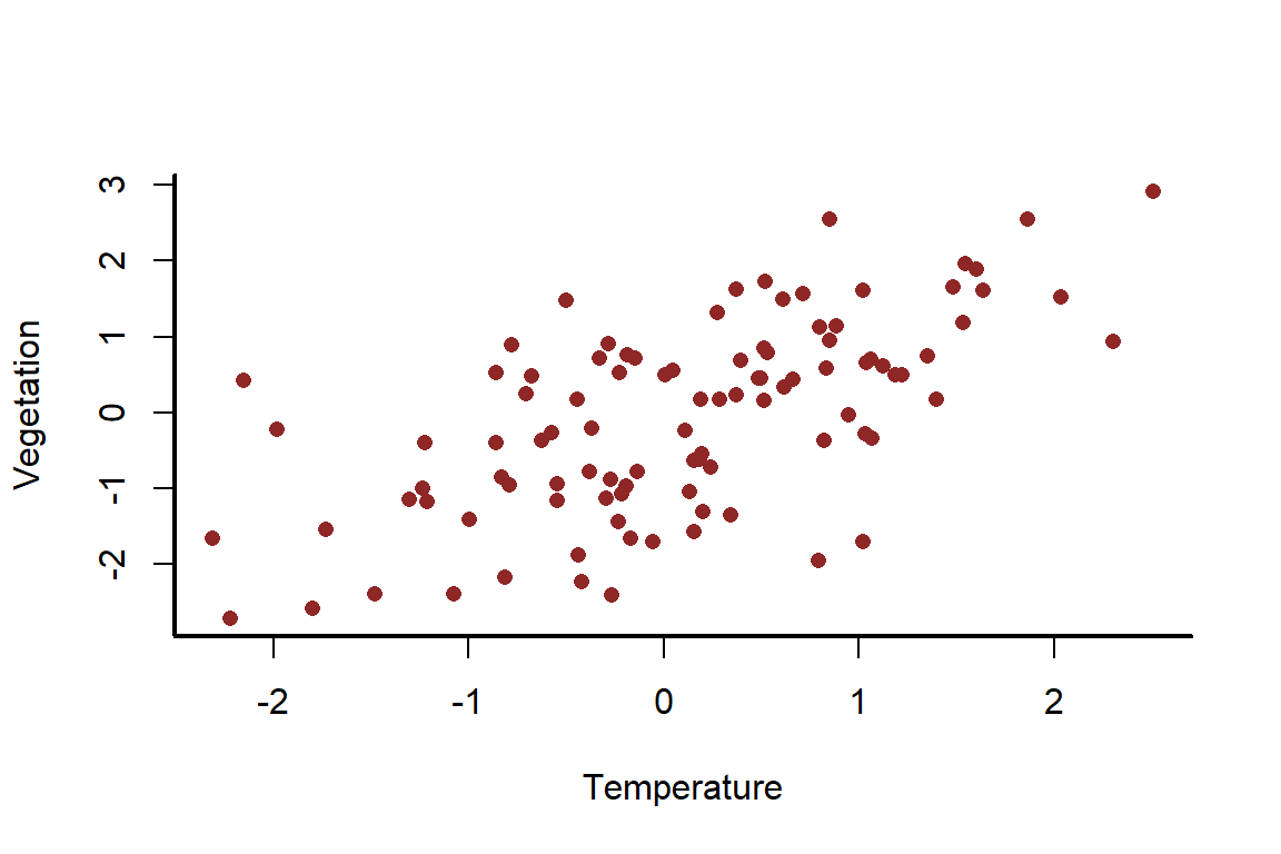
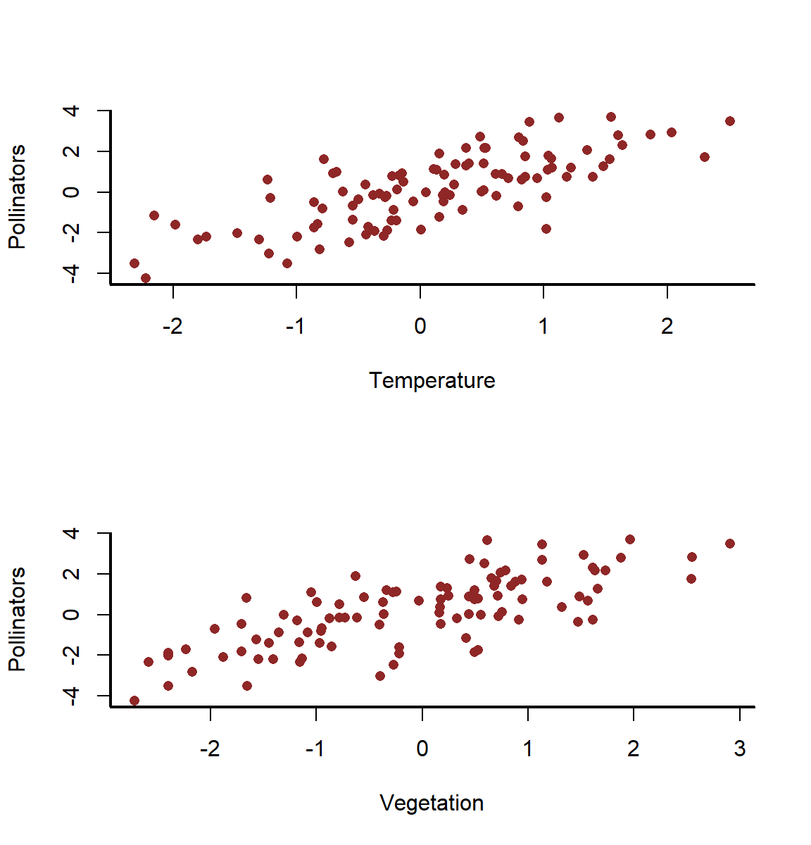
But this time, \(temperature\) also influences \(pollinator density\)
beta_temp_pollinators <- 0.75
And \(vegetation\), our outcome of interest, equally influences \(pollinator density\)
beta_veg_pollinators <- 0.75
The problem here is that pollinators now exists as a collider variable; both our outcome of interest and one of our predictors influences this variable. This is an all-too-common issue we are faced with in regressin modelling
pollinators <- rnorm(N,
                     mean = beta_temp_pollinators * temperature +
                       beta_veg_pollinators * vegetation,
                     sd = 1)
There are now strong apparent relationships all around
layout(matrix(1:2, nrow = 2))
myscatter(x = temperature,
          y = pollinators,
          xlab = 'Temperature',
          ylab = 'Pollinators')
myscatter(x = vegetation,
          y = pollinators,
          xlab = 'Vegetation',
          ylab = 'Pollinators')
layout(1)
If we thought that pollinator density could be a reasonable predictor of vegetation, the standard approach we would often take would be to fit univariate models for each of our predictors and then choose which ones to include in a final model based on some arbitrary significance threshold. Let’s see what happens if we do this
temp_only <- lm(vegetation ~ temperature)
summary(temp_only)
##
## Call:
## lm(formula = vegetation ~ temperature)
##
## Residuals:
##      Min       1Q   Median       3Q      Max
## -2.44451 -0.69136  0.03974  0.65918  2.26335
##
## Coefficients:
##             Estimate Std. Error t value Pr(>|t|)
## (Intercept) -0.14338    0.09937  -1.443    0.152
## temperature  0.79203    0.09952   7.959 3.11e-12 ***
## ---
## Signif. codes:  0 '***' 0.001 '**' 0.01 '*' 0.05 '.' 0.1 ' ' 1
##
## Residual standard error: 0.9885 on 98 degrees of freedom
## Multiple R-squared:  0.3926,	Adjusted R-squared:  0.3864
## F-statistic: 63.34 on 1 and 98 DF,  p-value: 3.106e-12
veg_only <- lm(vegetation ~ pollinators)
summary(veg_only)
##
## Call:
## lm(formula = vegetation ~ pollinators)
##
## Residuals:
##      Min       1Q   Median       3Q      Max
## -1.94531 -0.57399 -0.06453  0.57038  1.91163
##
## Coefficients:
##             Estimate Std. Error t value Pr(>|t|)
## (Intercept) -0.15133    0.08499  -1.781   0.0781 .
## pollinators  0.53784    0.04864  11.057   <2e-16 ***
## ---
## Signif. codes:  0 '***' 0.001 '**' 0.01 '*' 0.05 '.' 0.1 ' ' 1
##
## Residual standard error: 0.846 on 98 degrees of freedom
## Multiple R-squared:  0.555,	Adjusted R-squared:  0.5505
## F-statistic: 122.2 on 1 and 98 DF,  p-value: < 2.2e-16
Both predictors are found to be significant in univariate models; the standard approach we are taught now is to include them both in a final multivariable model
final_mod <- lm(vegetation ~ temperature + pollinators)
summary(final_mod)
##
## Call:
## lm(formula = vegetation ~ temperature + pollinators)
##
## Residuals:
##     Min      1Q  Median      3Q     Max
## -1.8385 -0.5926 -0.0930  0.5014  1.8816
##
## Coefficients:
##             Estimate Std. Error t value Pr(>|t|)
## (Intercept) -0.15736    0.08454  -1.861   0.0657 .
## temperature  0.19296    0.12839   1.503   0.1361
## pollinators  0.45497    0.07333   6.205 1.35e-08 ***
## ---
## Signif. codes:  0 '***' 0.001 '**' 0.01 '*' 0.05 '.' 0.1 ' ' 1
##
## Residual standard error: 0.8407 on 97 degrees of freedom
## Multiple R-squared:  0.5652,	Adjusted R-squared:  0.5562
## F-statistic: 63.04 on 2 and 97 DF,  p-value: < 2.2e-16
This model is supported by AIC over the simpler models. The lower the AIC, the better are the penalized in-sample predictions from the model
c('full model better',
  'temp only better',
  'veg only better')[which.min(c(AIC(final_mod),
                                 AIC(temp_only),
                                 AIC(veg_only)))]
## [1] "full model better"
A type II ANOVA reveals that if we wanted the most parsimonious model, we’d be justified in dropping \(temperature\) (even though this is the effect we actually care about!)
drop1(final_mod, test = 'F')
## Single term deletions
##
## Model:
## vegetation ~ temperature + pollinators
##             Df Sum of Sq    RSS     AIC F value    Pr(>F)
## <none>                   68.551 -31.759
## temperature  1    1.5962 70.147 -31.457  2.2586    0.1361
## pollinators  1   27.2062 95.757  -0.335 38.4969 1.349e-08 ***
## ---
## Signif. codes:  0 '***' 0.001 '**' 0.01 '*' 0.05 '.' 0.1 ' ' 1
In fact, just about any model selection routine you use on these data will favour the multivariable model (stepwise selection, ridge regression, LASSO etc….). But why do these general model selection routines favour a model that discards \(temperature\). How does the estimated effect of temperature on vegetation resemble what we simulated as the actual truth?
confint(final_mod)[2,]
##       2.5 %      97.5 %
## -0.06186813  0.44778663
beta_temp
## [1] 0.75
It misses. Badly. This is because of the influence of collider bias. We must be very cautious when throwing all sorts of variables into models and assuming the resulting estimates can be interpreted in any meaningful way. The correct approach here would actually be to omit \(pollinators\) altogether. This is better for inference, even though it doesn’t fit the data as well. We’ve already done that in our temp_only model
confint(temp_only)[2,]
##     2.5 %    97.5 %
## 0.5945409 0.9895126
beta_temp
## [1] 0.75
Effects are often estimated with more precision when including other predictors
Here we will explore why it is often important to adjust for other variables when estimating effects, even if those other variables are not “significant”. Simulate a scenario where age and season show independent effects on some disease’s infection probability
set.seed(5555)
N <- 200
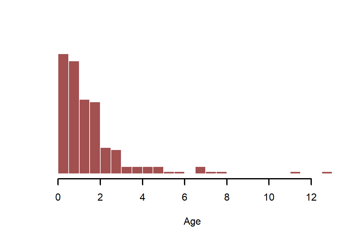
Simulate \(age\) as a log-normally distributed, positive continuous variable
age <- rlnorm(N)
myhist(age, xlab = 'Age')
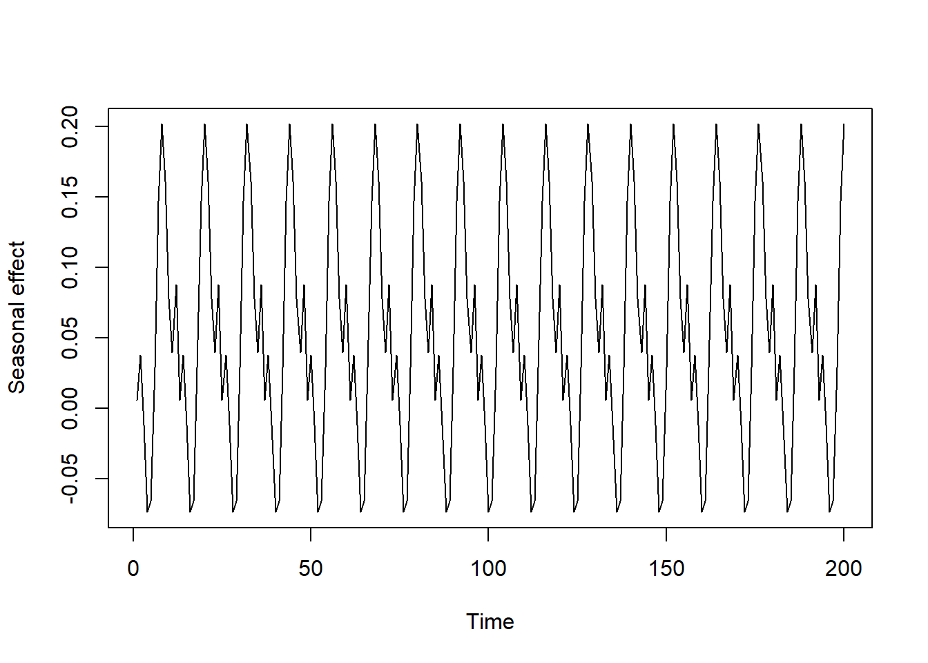
Simulate a cyclic seasonal pattern to replicate what we often see with transmittable diseases, which is a fairly strong and consistent variation in risk across seasons. This type of simulation can be done with combinations of sine and cosine functions
season_function <- rep((sin(0.2 * 1:12) - cos(-0.2 * 1:12) + sin(1:12)),
                        50)[1:N] * 0.1
plot(season_function, type = 'l',
     xlab = 'Time', ylab = 'Seasonal effect')
Convert season to a numeric indicator of month, just like we would use in a model
season <- rep(1:12, ceiling(N / 12))[1:N]
head(season, 24)
## [1] 1 2 3 4 5 6 7 8 9 10 11 12 1 2 3 4 5 6 7 8 9 10 11 12
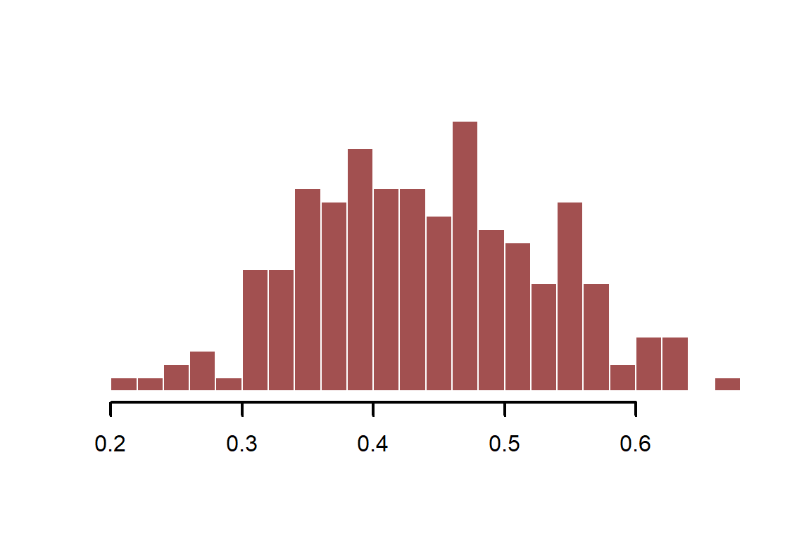
Calculate infection probability with an \(age\) effect of -0.4 (on the log scale) and with a minor seasonal effect. We use the plogis function, which uses the inverse logit transformation to convert real-valued continuous variables to the probability scale. This is the same link function that is used in logistic regression (where the outcomes are 1s and 0s) and in Beta regression (where the outcome is a proportion on (1,0)). We will use Beta regression here, which assumes the following:
$$\boldsymbol{inf~prob}\sim \text{Beta}(logit^{-1}(\mu)*\phi,(1-logit^{-1}(\mu))*\phi)$$
$$\mu={\alpha}+{\beta_{age}}*\boldsymbol{log(age)}+f(season)$$
Where \(\phi\) is a shape parameter that controls the spread of the distribution. We can use plogis to convert our simulated values from the real line to the probability scale (this is a fast and efficient version of inverse logit)
beta_logage <- -0.4
inf_prob <- plogis(-0.3 + season_function + beta_logage * log(age))
myhist(inf_prob)
Fit a beta regression model that ignores season
library(mgcv)
## Loading required package: nlme
## This is mgcv 1.8-42. For overview type 'help("mgcv-package")'.
mod_noseason <- gam(inf_prob ~ log(age),
                    family = betar(),
                    method = 'REML')
The estimate for \(log(age)\) is fairly precise
summary(mod_noseason)
##
## Family: Beta regression(605.665)
## Link function: logit
##
## Formula:
## inf_prob ~ log(age)
##
## Parametric coefficients:
##              Estimate Std. Error z value Pr(>|z|)
## (Intercept) -0.247234   0.005879  -42.05   <2e-16 ***
## log(age)    -0.390477   0.006448  -60.56   <2e-16 ***
## ---
## Signif. codes:  0 '***' 0.001 '**' 0.01 '*' 0.05 '.' 0.1 ' ' 1
##
##
## R-sq.(adj) =  0.951   Deviance explained = 95.2%
## -REML = -493.13  Scale est. = 1         n = 200
Fit a model that includes only \(season\), which finds that this predictor is not statistically significant on its own. Again, the standard practice would be to drop this predictor when we proceed with a multivariable analysis
mod_seasononly <- gam(inf_prob ~ s(season, bs = 'cc'),
                    family = betar(),
                    method = 'REML')
summary(mod_seasononly)
##
## Family: Beta regression(29.583)
## Link function: logit
##
## Formula:
## inf_prob ~ s(season, bs = "cc")
##
## Parametric coefficients:
##             Estimate Std. Error z value Pr(>|z|)
## (Intercept) -0.24268    0.02574  -9.429   <2e-16 ***
## ---
## Signif. codes:  0 '***' 0.001 '**' 0.01 '*' 0.05 '.' 0.1 ' ' 1
##
## Approximate significance of smooth terms:
##                 edf Ref.df Chi.sq p-value
## s(season) 0.0004364      8      0   0.607
##
## R-sq.(adj) =  5.21e-08   Deviance explained = 0.000239%
## -REML = -196.38  Scale est. = 1         n = 200
Fit a model that includes both predictors
mod_bothpredictors <- gam(inf_prob ~ log(age) + s(season, bs = 'cc'),
                    family = betar(),
                    method = 'REML')
The estimate for log(age) also appears precise in this model, just like in the first model
summary(mod_bothpredictors)
##
## Family: Beta regression(14453.538)
## Link function: logit
##
## Formula:
## inf_prob ~ log(age) + s(season, bs = "cc")
##
## Parametric coefficients:
##              Estimate Std. Error z value Pr(>|z|)
## (Intercept) -0.247699   0.001206  -205.5   <2e-16 ***
## log(age)    -0.399987   0.001343  -297.9   <2e-16 ***
## ---
## Signif. codes:  0 '***' 0.001 '**' 0.01 '*' 0.05 '.' 0.1 ' ' 1
##
## Approximate significance of smooth terms:
##             edf Ref.df Chi.sq p-value
## s(season) 7.748      8   4518  <2e-16 ***
## ---
## Signif. codes:  0 '***' 0.001 '**' 0.01 '*' 0.05 '.' 0.1 ' ' 1
##
## R-sq.(adj) =  0.998   Deviance explained = 99.8%
## -REML = -787.93  Scale est. = 1         n = 200
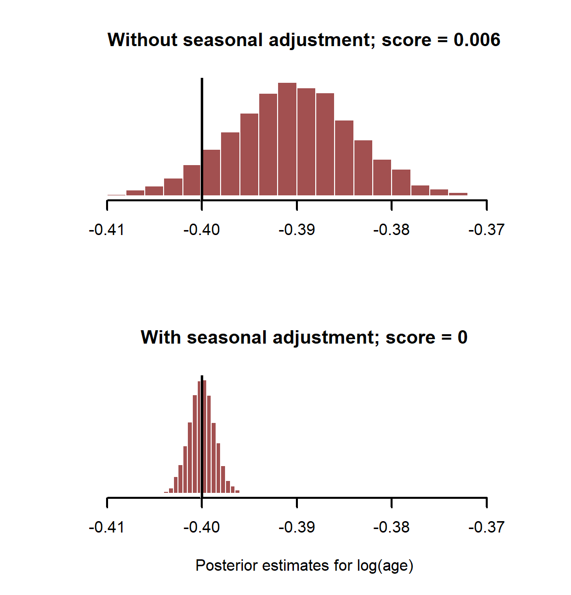
But which model gives us better estimates for log(age)? Draw 5,000 posterior estimates from each model’s posterior coefficient distribution. Because gam() uses a form of maximum likelihood for estimation, the posterior once again is an implied multivariate Gaussian. The variance-covariance matrix for the coefficients is stored in the model object in the Vc slot
coefs_noseason <- MASS::mvrnorm(5000, mu = coef(mod_noseason),
                       Sigma = mod_noseason$Ve)
coefs_bothpredictors <- MASS::mvrnorm(5000, mu = coef(mod_bothpredictors),
                                Sigma = mod_bothpredictors$Ve)
Calculate the continuous rank probability score (CRPS), a proper scoring rule for probabilistic predictions; a lower score is better, as it indicates the probability density is more concentrated around the true value
if(!require(scoringRules)){
  install.packages('scoringRules')
}
## Loading required package: scoringRules
## Warning: package 'scoringRules' was built under R version 4.3.2
score_noseason <- scoringRules::crps_sample(y = beta_logage,
                                            dat = t(coefs_noseason[,2]))
score_bothpredictors <- scoringRules::crps_sample(y = beta_logage,
                                              dat = t(coefs_bothpredictors[,2]))
Plot estimates and print the CRPS for each model
layout(matrix(1:2, nrow = 2))
myhist(coefs_noseason[,2],
       xlim = range(c(coefs_noseason[,2], coefs_bothpredictors[,2])),
       main = paste0('Without seasonal adjustment; score = ', round(score_noseason, 3)))
abline(v = beta_logage, lwd = 3, col = 'white')
abline(v = beta_logage, lwd = 2.5)

myhist(coefs_bothpredictors[,2], xlab = 'Posterior estimates for log(age)',
            xlim = range(c(coefs_noseason[,2], coefs_bothpredictors[,2])),
       main = paste0('With seasonal adjustment; score = ', round(score_bothpredictors, 3)))
abline(v = beta_logage, lwd = 3, col = 'white')
abline(v = beta_logage, lwd = 2.5)
layout(1)
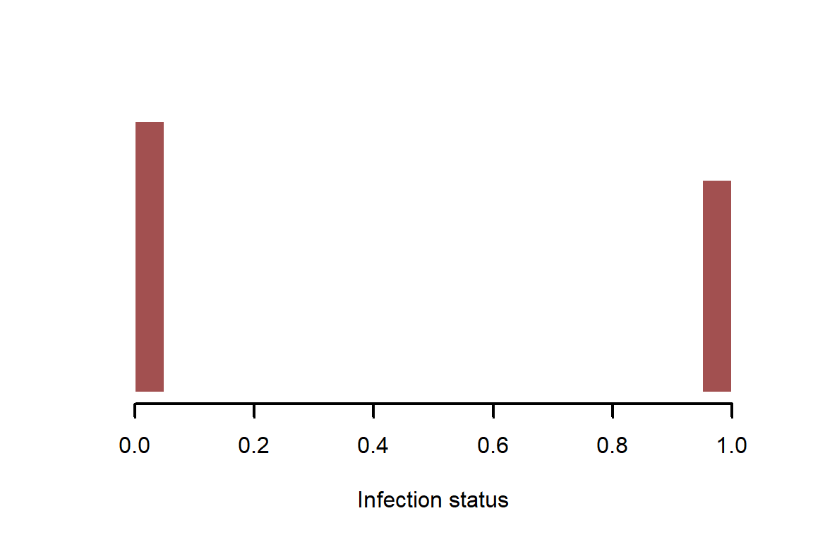
Here it is clear that adjusting for important control variables, even if they aren’t “significant”, gives us better estimates of risk factors. What happens if we have binary outcomes as our dependent variable? This is often the case in disease surveillance. We can easily generate such data using another of R’s random number generator functions. See ?rbinom for more details
infections <- rbinom(n = N, size = 1, prob = inf_prob)
myhist(infections, xlab = 'Infection status')
Fit the same models as above, but this time use a Bernoulli observation model with logit link function. The full model we will fit is:
$$\boldsymbol{infections}\sim \text{Bernoulli}(p)$$
$$logit(p)={\alpha}+{\beta_{age}}*\boldsymbol{log(age)}+f(season)$$
mod_noseason <- gam(infections ~ log(age),
                    family = binomial(),
                    method = 'REML')
summary(mod_noseason)
##
## Family: binomial
## Link function: logit
##
## Formula:
## infections ~ log(age)
##
## Parametric coefficients:
##             Estimate Std. Error z value Pr(>|z|)
## (Intercept)  -0.2423     0.1434  -1.689   0.0912 .
## log(age)     -0.2517     0.1549  -1.625   0.1043
## ---
## Signif. codes:  0 '***' 0.001 '**' 0.01 '*' 0.05 '.' 0.1 ' ' 1
##
##
## R-sq.(adj) =  0.00824   Deviance explained = 0.98%
## -REML = 137.81  Scale est. = 1         n = 200
mod_seasononly <- gam(infections ~ s(season, bs = 'cc'),
                    family = binomial(),
                    method = 'REML')
summary(mod_seasononly)
##
## Family: binomial
## Link function: logit
##
## Formula:
## infections ~ s(season, bs = "cc")
##
## Parametric coefficients:
##             Estimate Std. Error z value Pr(>|z|)
## (Intercept)  -0.2490     0.1449  -1.718   0.0858 .
## ---
## Signif. codes:  0 '***' 0.001 '**' 0.01 '*' 0.05 '.' 0.1 ' ' 1
##
## Approximate significance of smooth terms:
##            edf Ref.df Chi.sq p-value
## s(season) 1.95      8  8.352 0.00572 **
## ---
## Signif. codes:  0 '***' 0.001 '**' 0.01 '*' 0.05 '.' 0.1 ' ' 1
##
## R-sq.(adj) =  0.0423   Deviance explained =  3.8%
## -REML = 135.62  Scale est. = 1         n = 200
mod_bothpredictors <- gam(infections ~ log(age) + s(season, bs = 'cc'),
                    family = binomial(),
                    method = 'REML')
summary(mod_bothpredictors)
##
## Family: binomial
## Link function: logit
##
## Formula:
## infections ~ log(age) + s(season, bs = "cc")
##
## Parametric coefficients:
##             Estimate Std. Error z value Pr(>|z|)
## (Intercept)  -0.2506     0.1461  -1.715   0.0863 .
## log(age)     -0.2722     0.1594  -1.708   0.0877 .
## ---
## Signif. codes:  0 '***' 0.001 '**' 0.01 '*' 0.05 '.' 0.1 ' ' 1
##
## Approximate significance of smooth terms:
##             edf Ref.df Chi.sq p-value
## s(season) 1.985      8  8.743 0.00475 **
## ---
## Signif. codes:  0 '***' 0.001 '**' 0.01 '*' 0.05 '.' 0.1 ' ' 1
##
## R-sq.(adj) =  0.0512   Deviance explained = 4.93%
## -REML = 135.02  Scale est. = 1         n = 200
coefs_noseason <- MASS::mvrnorm(5000, mu = coef(mod_noseason),
                       Sigma = mod_noseason$Ve)
coefs_bothpredictors <- MASS::mvrnorm(5000, mu = coef(mod_bothpredictors),
                                Sigma = mod_bothpredictors$Ve)
score_noseason <- scoringRules::crps_sample(y = beta_logage,
                                            dat = t(coefs_noseason[,2]))
score_bothpredictors <- scoringRules::crps_sample(y = beta_logage,
                                              dat = t(coefs_bothpredictors[,2]))
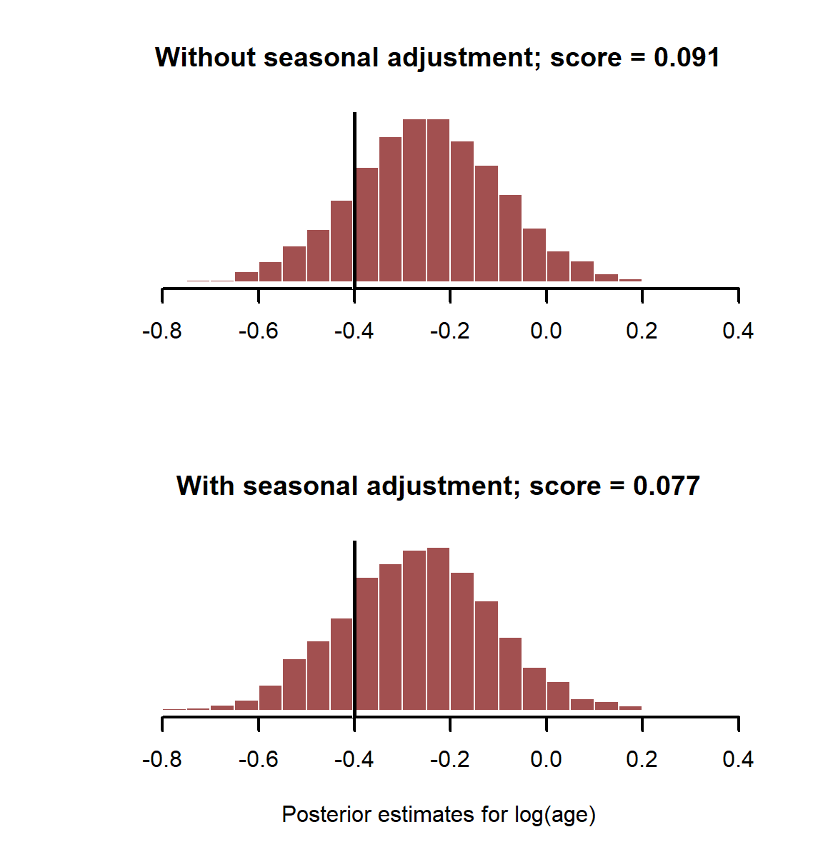
Plot estimates and print the CRPS for each model
layout(matrix(1:2, nrow = 2))
myhist(coefs_noseason[,2],
       xlim = range(c(coefs_noseason[,2], coefs_bothpredictors[,2])),
       main = paste0('Without seasonal adjustment; score = ', round(score_noseason, 3)))
abline(v = beta_logage, lwd = 3, col = 'white')
abline(v = beta_logage, lwd = 2.5)

myhist(coefs_bothpredictors[,2], xlab = 'Posterior estimates for log(age)',
            xlim = range(c(coefs_noseason[,2], coefs_bothpredictors[,2])),
       main = paste0('With seasonal adjustment; score = ', round(score_bothpredictors, 3)))
abline(v = beta_logage, lwd = 3, col = 'white')
abline(v = beta_logage, lwd = 2.5)
layout(1)
In this case it doesn’t make much difference whether we adjust for \(season\) or not when estimating effect of log(age). This is because binary data has much less information than the proportional data we were using in the Beta regression. We’d need to boos our sample size to have a better chance of adequately estimating these effects with a logistic regression. This is another advantage of simulation, as it allows us to get a better sense of the limitations of our sampling designs
Failing to account for unobserved autocorrelation causes problems
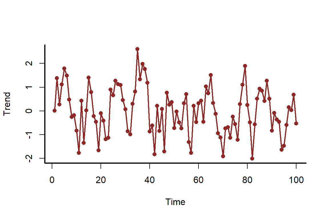
In this final example, we will simulate a time series of counts that has autocorrelation in the underlying data-generating process. It is useful to get a sense of how models perform when we fail to take this autocorrelation into account. First we simulate the underlying autocorrelated trend, which follows an AR1 model
set.seed(500)
N <- 100
time <- 1:N
trend <- as.vector(scale(arima.sim(model = list(ar = 0.7), n = N)))
myscatter(x = time, y = trend, xlab = 'Time', ylab = 'Trend')
lines(trend, col = c_dark, lwd = 2)
Next we simulate our covariate, \(rainfall\), and it’s linear additive coefficient
rainfall <- rnorm(N)
beta_rain <- 0.4
Finally, we can simulate the counts. In this case, counts follow a Poisson observation process. Poisson regression that assumes the underlying mean evolves on the log scale:
$$\boldsymbol{Counts}\sim \text{Poisson}(\lambda)$$
$$log(\lambda)={\alpha}+{\beta_{rainfall}}*\boldsymbol{rainfall}+trend$$
In this example, the linear predictor, \(log(\lambda)\) (referred to here as \(\mu\)), captures the additive effects of the intercept \(\alpha\), the effect of \(rainfall\) and the underlying trend on the the log of the mean for \(counts\). See ?rpois for more information about the Poisson distribution functions in R
alpha <- 1
mu <- alpha + beta_rain * rainfall + 0.8 * trend
counts <- rpois(n = N, lambda = exp(mu))
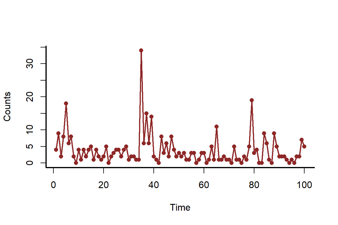
Plot the counts over time
myscatter(x = time, y = counts, xlab = 'Time', ylab = 'Counts')
lines(counts, col = c_dark, lwd = 2)
When working with time series, it is always useful to understand whether there is any autocorrelation in the observations. This can be checked using the acf() function
acf(counts)
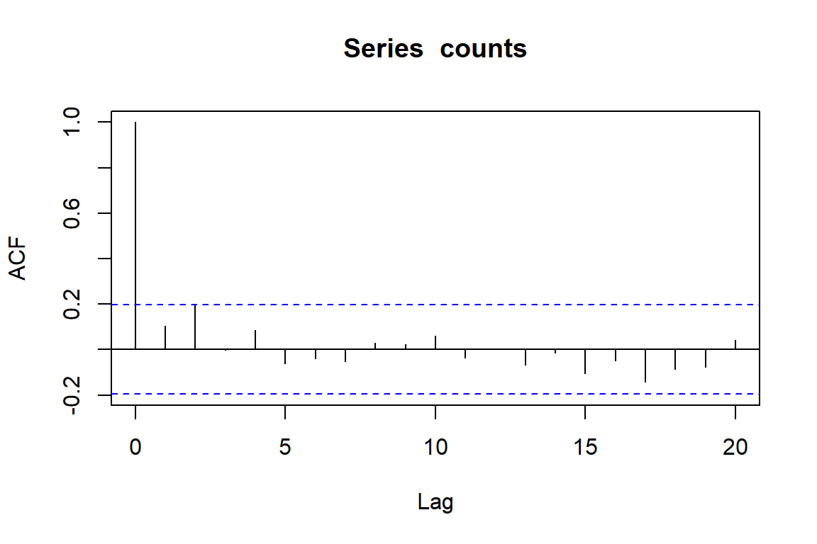
This doesn’t give us too much concern, and many people would use the fact that none of the lags shows too much autocorrelation as evidence that they do not need to account for this in their models. But what happens when we ignore time in our models?
mod_notime <- gam(counts ~ rainfall,
                   family = poisson())
acf(residuals(mod_notime))
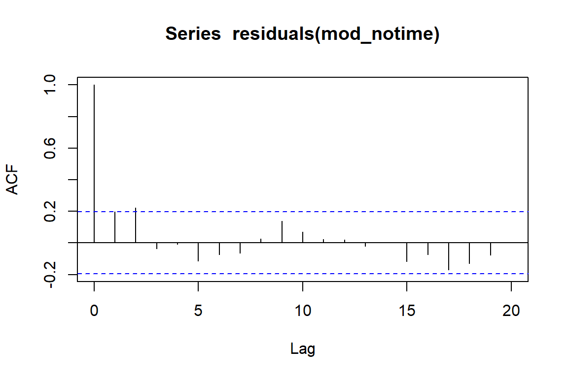
There is some apparent autocorrelation left in the residuals. This means our model’s errors are not independent, which is a violation of the model’s assumptions. This can lead to overly precise standard errors and overconfident p-values. But it can also lead to downright absurd estimates for our predictors. Let’s compare estimates of the \(rainfall\) coefficient from this model with a model that does attempt to capture the effect of time. This is done using a flexible smoothing spline for time
mod_time <- gam(counts ~ rainfall + s(time, k = 30),
                     family = poisson())
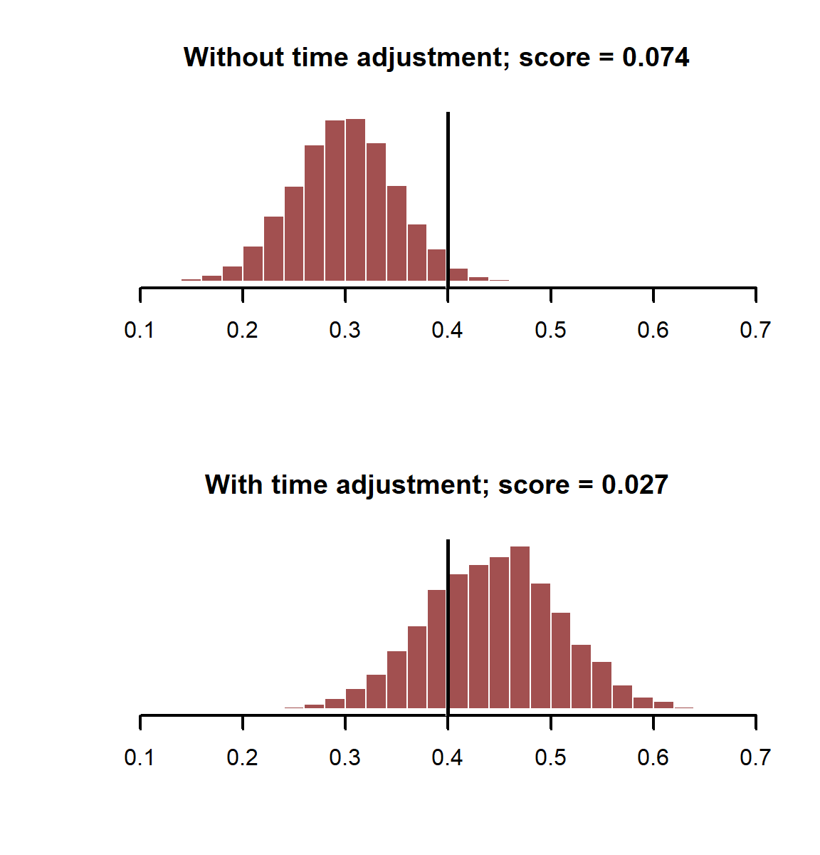
As before, we can compare the accuracies of our posterior estimates of the \(rainfall\) coefficient using probabilistic scoring rules
coefs_notime<- MASS::mvrnorm(5000, mu = coef(mod_notime),
                                Sigma = mod_notime$Ve)
coefs_time <- MASS::mvrnorm(5000, mu = coef(mod_time),
                                      Sigma = mod_time$Ve)

score_notime <- scoringRules::crps_sample(y = beta_rain,
                                            dat = t(coefs_notime[,2]))
score_time<- scoringRules::crps_sample(y = beta_rain,
                                                  dat = t(coefs_time[,2]))

layout(matrix(1:2, nrow = 2))
myhist(coefs_notime[,2],
       xlim = range(c(coefs_notime[,2], coefs_time[,2])),
       main = paste0('Without time adjustment; score = ', round(score_notime, 3)))
abline(v = beta_rain, lwd = 3, col = 'white')
abline(v = beta_rain, lwd = 2.5)
myhist(coefs_time[,2],
       xlim = range(c(coefs_notime[,2], coefs_time[,2])),
       main = paste0('With time adjustment; score = ', round(score_time, 3)))
abline(v = beta_rain, lwd = 3, col = 'white')
abline(v = beta_rain, lwd = 2.5)
layout(1)
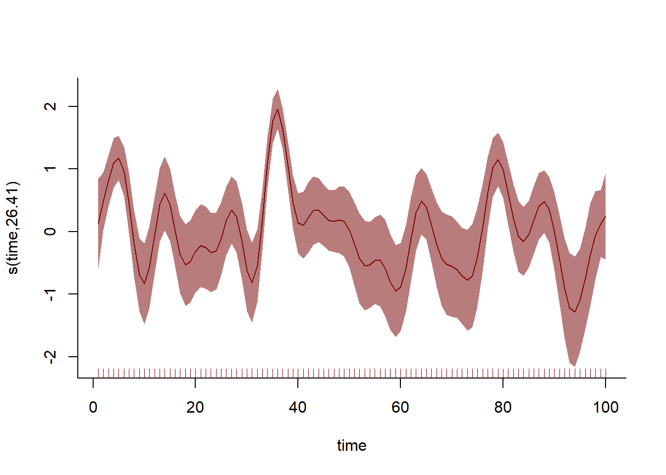
The model with the temporal component does better in this case, giving us more accurate estimates of our coefficient of interest. How does the smoothing spline capture this temporal variation?
plot(mod_time, shade = TRUE, shade.col = c_mid, col = c_dark_highlight,
     bty = 'l')
More examples will follow, but now that you have the building blocks of simulation of random variables and random sampling, you can simulate more complex generative models directly